Bernoulli experiments in stan
I’m a big fan of expressing math as code. While it’s not as terse, I think it’s a lot easier to use to learn statistics. In this post I’ll break down a small set (three!) bernoulli experiments. Binary data is really common in business, so it pays to work through the details.
At the end I’ll use stan to generate a probablistic estimate of \(\hat{p}\). Markov chain monte carlo is overkill for this type of problem (see relative likelihood), but in order to learn I find it’s best to start with simple things.
library(rstan)
library(dplyr)
rstan_options(auto_write = TRUE)
options(mc.cores = parallel::detectCores())
First, I’ll generate three bernoulli experiments with pretend “true” parameter values,
dbernoulli <- function(x, p) dbinom(x, 1, p)
rbernoulli <- function(n, p) rbinom(n, 1, p)
set.seed(1)
N <- 3L # L means integer in R
(p <- runif(1))
## [1] 0.2655087(coin_flips <- rbernoulli(N, p))## [1] 0 0 1spineplot(table(coin_flips == 1, coin_flips == 0), axes = FALSE,
main = "My observed coin flip proportions")
Now let’s check that I didn’t make a mistake generating the data by calculating the maximum likelihood estimate (a process I’m more familiar with),
bernoulli pdf(my random variable; true unknown probability) = p^x_i * (1 - p)^ 1-x_iThis could be written more compactly like,
\(f(x; p) = p^x \times (1 - p)^{n-x}\) where x can only take the values 0 or 1 and \(0 < p < 1\) strictly.
The most crucial part of doing high quality statistics is to understand how to create and calculate a function that is at worst proportional to the probability of the observed data. The fact that this function, if constructed, is proportional to the probability of the observed data makes the function operate as a lens. If you like music, the ability to calculate this function is similar to having a high-quality needle on a record player. While this lens can be improved (by incorporating more information), on its own it’s extremely high quality. This function is the likelihood function.
How do we get it? Easy! We evaluate \(f(x; p)\) at each data point starting with the first and then multiply the terms. So let’s do it!
Remember our coin flips,
coin_flips## [1] 0 0 1Let’s take the first,
function(p) { dbinom(coin_flips[1], p) } # <--- first flip was 0## function(p) { dbinom(coin_flips[1], p) }Remember a function is what’s returned! Now let’s evaluate the density at the next two data points,
function(p) { dbinom(coin_flips[2], p) } # <--- 2nd flip was 0## function(p) { dbinom(coin_flips[2], p) }function(p) { dbinom(coin_flips[3], p) } # <--- 3rd flip was 1## function(p) { dbinom(coin_flips[3], p) }Two more functions. Now we multiply them, but in order to make this possible we refactor a little. That is we factor out \(p\) to just one function,
bernoulli_likelihood <- function(p_to_try) {
  prod((function() { dbernoulli(coin_flips[1], p_to_try) })(),
       (function() { dbernoulli(coin_flips[2], p_to_try) })(),
       (function() { dbernoulli(coin_flips[3], p_to_try) })())
}
We have our likelihood function, woo! Now, let’s try some values,
bernoulli_likelihood(p_to_try = 0.0001)## [1] 9.998e-05Wow, although I know that this isn’t the probability of the observed data, I do know that it’s proportional to the data. 9.998e-05 seems quite small for something that is necessarily positive. Now I can see that 0.0001 was a silly first choice, I could use bisection to do this quicker,
bernoulli_likelihood(p_to_try = 0.5)## [1] 0.125Cool! Now I’m not sure which side has the more likely value, let’s just choose the low end and try bisection again (between 0 and 0.5),
bernoulli_likelihood(p_to_try = 0.25)## [1] 0.140625Ah! 0.25 is a better estimate of p than 0.5. Let’s try 0.5 + 0.25 / 2, 0.375,
bernoulli_likelihood(p_to_try = 0.375)## [1] 0.1464844Ah even higher! Repeat repeat repeat (or revert to a terser syntax to do algebra aka typical math syntax, see “maximum likelihood estimation”).
bernoulli_likelihood(p_to_try = 0.315)## [1] 0.1478059bernoulli_likelihood(p_to_try = 0.345)## [1] 0.1480136bernoulli_likelihood(p_to_try = 0.33)## [1] 0.148137bernoulli_likelihood(p_to_try = 0.3375)## [1] 0.1481309Ah, we found a lower value! So we can fall back to 0.33. I’m sure this function could be written recursively. I’ll leave that to myself for a future exercise. :)
To recap, we generated a pretend “true” \(\hat{p}\) that was 0.2655087. We in essence “hid” this value from ourselves and generated three bernoulli experiments that yielded 0 0 1. From this observed data we were able to estimate \(\hat{p}\) as 0.33, not exactly 0.26 but also not bad for only observing three data points! One can always complain that their sample size isn’t large enough, but a smarter alternative is to become really good at squeezing the most information out of the least data!
Now that we feel pretty confident that ~ 0.33 maximizes the thing that’s proportional to the probability of the observed data at worst (at best it is equal to the probability of the observed data), let’s use the opportunity to learn some stan,
model_code <- "
data {
  int N;
  int y[N];
}
parameters {
  real<lower=0,upper=1> p;
}
model {
  y ~ bernoulli(p);
}"extract(fit, pars = "p") %>% unlist() %>% density() %>%
plot(main = "Posterior density of p")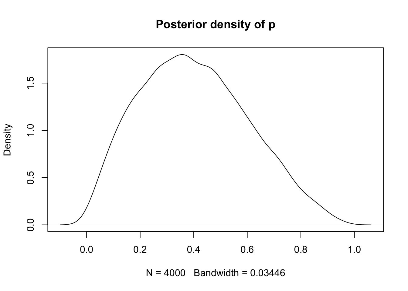
Thanks for following along! For a more efficient and much computationally cheaper way to compute this particular interval see relative likelihood.
P.S. — I have to say that this post is heavily inspired by the great work of my advisor and his co-authors! He taught me that no sample is too small to extract info from!