Geometric distribution and Bayesian updating
The concept of Bayesian updating is so fascinating: encode information using a likelihood and readily update the likelihood with each subsequent data point. In this manner the “prior” (what we have seen and therefore believe encoded) and likelihood (our “story”) are an engine for producing posterior distributions.
Firing the engine and producing posteriors ranges from very easy and computationally cheap to very computationally intensive.
Certain distributions have so-called conjugate priors. These are distributions whose likelihood functions are proportional to each other constants aside. Using the property of conjugacy enables very computationally cheap updating in contrast to Markov Chain Monte Carlo.
The so-called counting distributions:
- Bernoulli
- Binomial
- Geometric
- Negative Binomial
all share the beta distribution as their conjugate prior. This means that we can directly update a beta distribution having observed a heads / tails type process while perserving the ability to analyze the data through the interpretive lens of any of these distributions.
Below I define such a process with a probability of heads on any given flip of 5 percent. I encode basically weak to no special belief of the “magical unknown parameter,” 5 percent.
set.seed(0)
magical_unknown_param <- 0.05
original_belief_a <- 1
original_belief_b <- 1
Now I draw one observation from a geometric distribution by flipping the coin until I see the first heads. The result is the number of tails I saw along the way,
(x <- rgeom(1, prob = magical_unknown_param))## [1] 4In this case it took four tails in a row before we observed the first heads. Let’s update our beliefs,
updated_belief_a <- original_belief_a + 1
updated_belief_b <- original_belief_b + sum(x)

(updated_beliefs <- rbeta(1, updated_belief_a, updated_belief_b))
## [1] 0.6236603Now I’ll repeat the process all at once,
(x <- c(x, rgeom(1, prob = magical_unknown_param)))## [1] 4 10(updated_belief_a <- original_belief_a + 1)## [1] 2(updated_belief_b <- original_belief_b + sum(x))## [1] 15(updated_beliefs <- rbeta(1, updated_belief_a, updated_belief_b))## [1] 0.02604405Again,
(x <- c(x, rgeom(1, prob = magical_unknown_param)))## [1] 4 10 37(updated_belief_a <- original_belief_a + 1)## [1] 2(updated_belief_b <- original_belief_b + sum(x))## [1] 52(updated_beliefs <- rbeta(1, updated_belief_a, updated_belief_b))## [1] 0.07199219Again,
(x <- c(x, rgeom(1, prob = magical_unknown_param)))## [1] 4 10 37 16(updated_belief_a <- original_belief_a + 1)## [1] 2(updated_belief_b <- original_belief_b + sum(x))## [1] 68(updated_beliefs <- rbeta(1, updated_belief_a, updated_belief_b))## [1] 0.02166169After repeating the process, I wanted to write a recursive function that would accept a geometric random variable outcome and use the conjugate prior to return an observation from the posterior distribution,
generate_posterior <- function(x, belief_a = 1, belief_b = 1, n = 1) {
  if(length(x) == 0) {
    message("beta(", belief_a, ", ", belief_b, ")")
    return(rbeta(1, belief_a, belief_b))
  } else {
    message("a is: ", belief_a, " b is: ", belief_b,
            " x is: ", head(x, 1), " n is: ", n,
            " Current belief is: ", round(rbeta(1, belief_a, belief_b), 2))
    generate_posterior(x = tail(x, -1),
                       belief_a = belief_a + 1,
                       belief_b = belief_b + head(x, 1),
                       n = n + 1)
  }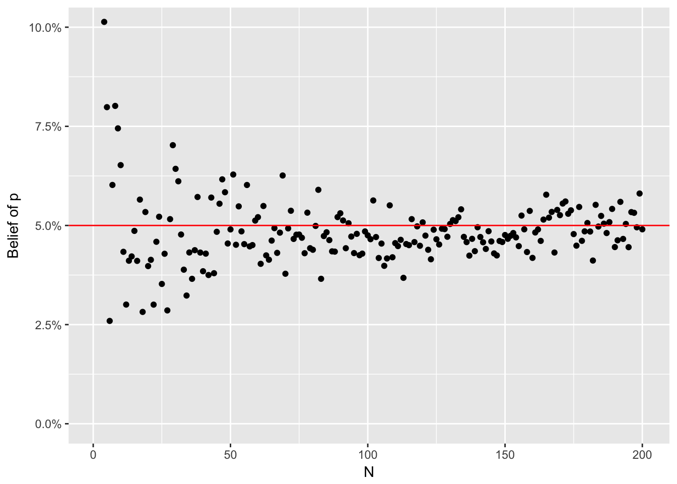
}generate_posterior(x = rgeom(10, 0.05), belief_a = 1, belief_b = 1)## a is: 1 b is: 1 x is: 1 n is: 1 Current belief is: 0.9## a is: 2 b is: 2 x is: 13 n is: 2 Current belief is: 0.51## a is: 3 b is: 15 x is: 28 n is: 3 Current belief is: 0.14## a is: 4 b is: 43 x is: 15 n is: 4 Current belief is: 0.06## a is: 5 b is: 58 x is: 7 n is: 5 Current belief is: 0.06## a is: 6 b is: 65 x is: 13 n is: 6 Current belief is: 0.06## a is: 7 b is: 78 x is: 2 n is: 7 Current belief is: 0.11## a is: 8 b is: 80 x is: 4 n is: 8 Current belief is: 0.14## a is: 9 b is: 84 x is: 7 n is: 9 Current belief is: 0.14## a is: 10 b is: 91 x is: 1 n is: 10 Current belief is: 0.09## beta(11, 92)## [1] 0.09739849Finally we can visualize the pre-specified “magical unknown parameter” against a set of draws from successively informed posterior distributions,
library(tidyverse)
tibble::tibble(x = rgeom(2e2, 0.05), a = 1, b = 1) %>%
  mutate(n = 1:n(), a = n + 1, b = cumsum(x) + 1) %>%
  rowwise() %>%
  mutate(belief = rbeta(1, a, b)) %>%
  ungroup() %>%
  ggplot(aes(x = n, y = belief)) +
  geom_point() +
  geom_hline(yintercept = 0.05, colour = "red") +
  coord_cartesian(ylim = c(0, 0.1)) +
  scale_y_continuous(labels = scales::percent) +
  ylab("Belief of p") +
  xlab("N")