Modeling subscription churn
Statwonk
May 22, 2016
Note: this is a work in progress please send feedback to @statwonk
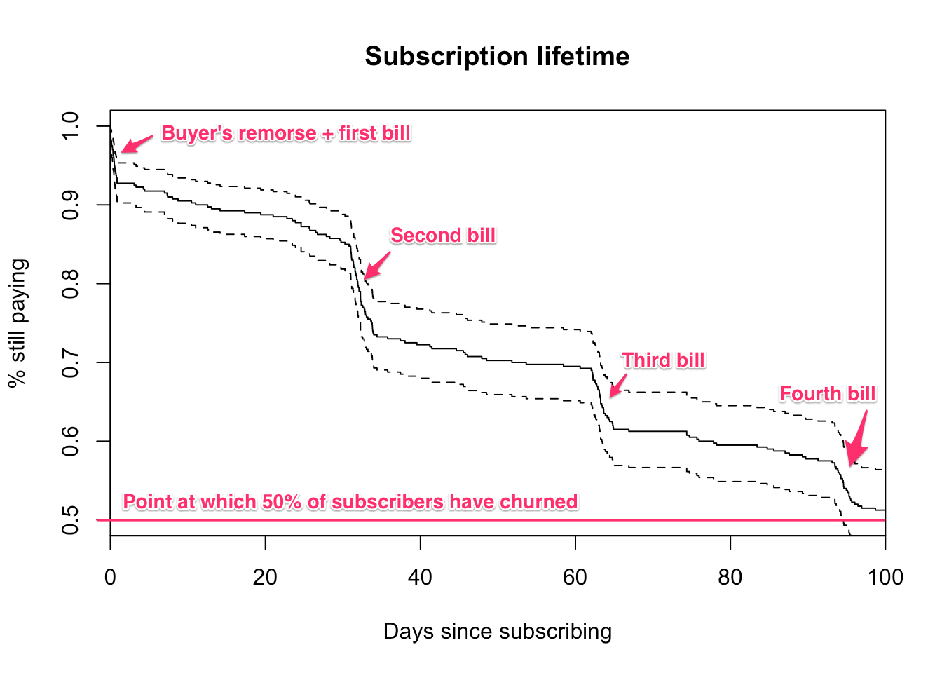
Subscription churn usually clusters around the first day and each subsequent bill. “Buyers remorse” is a common phrase for early churn and it’s no surprise that subscribers churn when presented with a bill. It’s important to model these clusters well because they’re where most customers churn.
Let’s generate some toy data reflecting this common business scenario.
library(eha)

example_hazard_rates <- c(
  0.06, # buyer's remorse
  0.003,
  0.055, # second bill
  0.002,
  0.05, # third bill
  0.002,
  0.04, # fourth bill
  0.004)

# It seems that the eha::rpch function has a little bug
# with failing to pass the cuts, levels params. This is
# a quick fix.

# First generate piecewise-constant survival data
rpch <- function(n, cuts, levels) {
  x <- runif(n)
  qpch(x, cuts, levels)
}

x <- data.frame(
  times = rpch(
    n = 400,
    cuts = c(1, # initial purchase
             31, 34, # second bill
             62, 65, # third bill
             93, 96 # fourth bill
    ),
    levels = example_hazard_rates
  ),
  censor = 1
)

plot(
  survfit(Surv(times, censor) ~ 1, data = x),
  xlim = c(0, 100),
  ylim = c(0.5, 1),
  conf.int = TRUE,
  main = "Subscription lifetime",
  ylab = "% still paying",
  xlab = "Days since subscribing"
)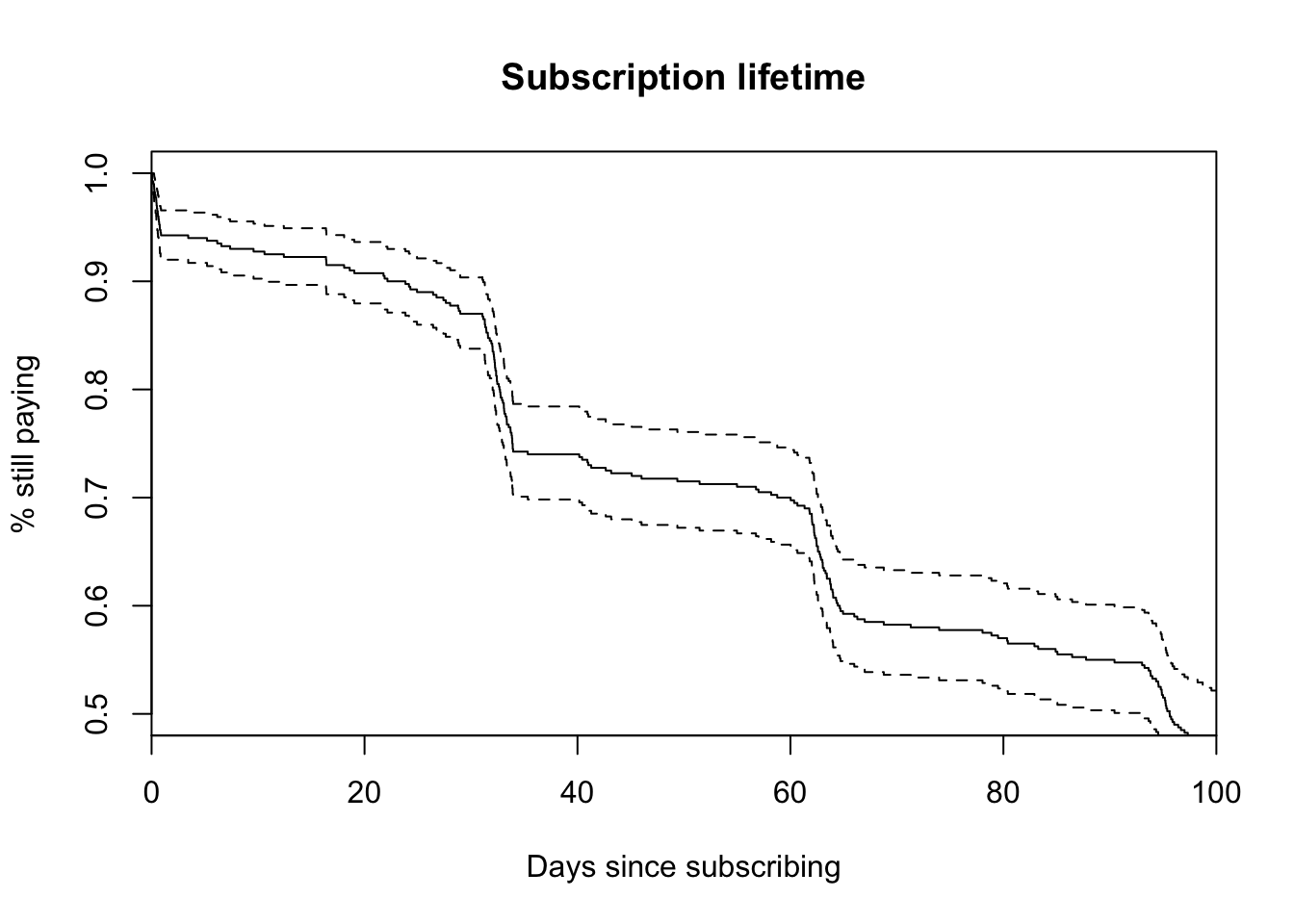
Alright, now we have our toy dataset.
Typical parametric models will fail in the face of buyer’s remorse and billing churn, so we need something new.
library(flexsurv) # <-- awesome library; Christopher Jackson, you rock!
fitg <- flexsurvreg(
  Surv(times, censor) ~ 1,
  data = x, dist = "gengamma")
plot(fitg, xlim = c(0, 100), ylim = c(0.5, 1),
     main = "Subscription lifetime",
     ylab = "% still paying",
     xlab = "Days since subscribing")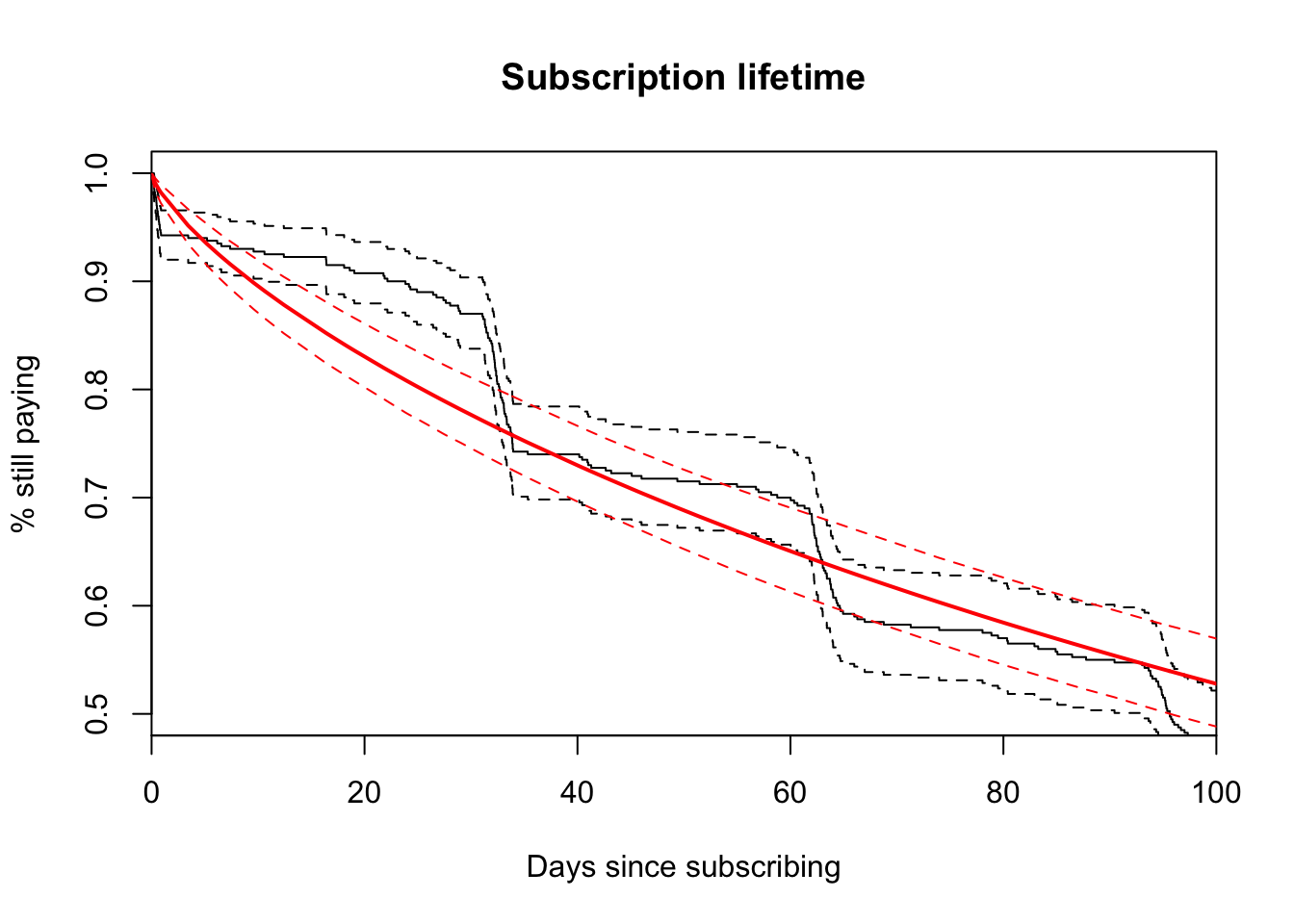
pfit <- phreg(
  Surv(times, censor) ~ 1, data = x,
  dist = "pch",
  cuts = c(1, # initial purchase
           31, 34, # second bill
           62, 65, # third bill
           93, 96 # fourth bill
  )
)
survival_estimates <- function(x, xlim = c(0, 100)) {
  if(x$n.strata > 1) stop("Developed for a single strata.")
  ncov <- length(x$means)
  npts <- 4999
  xx <- seq(xlim[[1]], xlim[[2]], length = npts)
  ppch(xx, x$cuts, x$hazards[1, ], lower.tail = FALSE)
}

estimates <- survival_estimates(pfit)
plot(fitg, xlim = c(0, 100), ylim = c(0.5, 1),
     main = "Subscription lifetime",
     ylab = "% still paying",
     xlab = "Days since subscribing")
lines(
  x = seq(0, 100, length = length(estimates)),
  y = estimates,
  col = "blue")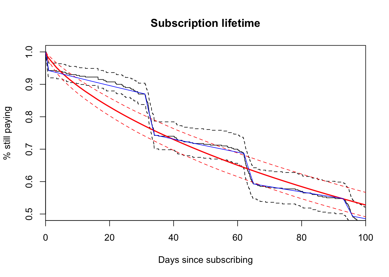
estimated_hazard_rates <- piecewise(
  enter = 0, exit = x$times, event = x$censor,
  cutpoints = c(1, # initial purchase
                31, 34, # second bill
                62, 65, # third bill
                93, 96 # fourth bill
  ))$intensity
… compare to our original example hazard rates,
data.frame(
  actual = round(example_hazard_rates, 3),
  estimates = round(example_hazard_rates, 3)
)
## actual estimates
## 1 0.060 0.060
## 2 0.003 0.003
## 3 0.055 0.055
## 4 0.002 0.002
## 5 0.050 0.050
## 6 0.002 0.002
## 7 0.040 0.040
## 8 0.004 0.004Perfect! We don’t need statistics! :-p Since we’re specificing the random data upfront, we’re able to choose perfect cut points from a known distribution. It’s no suprise the model fits very well. In reality, we need to take this a step further by bootstrapping the estimates for a measure of uncertainty similar to our plotted parametric model. This is what we’ll want to deploy on our actual churn data.
piecewise_fit <- function(d, i) {
  survival_estimates(
    phreg(
      Surv(times, censor) ~ 1, data = d[i, ],
      dist = "pch",
      cuts = c(1, # initial purchase
               31, 34, # second bill
               62, 65, # third bill
               93, 96 # fourth bill
      )
    )
  )
}
library(boot)
library(dplyr)
library(reshape2)
pch_estimates <- t(boot(x, piecewise_fit, R = 100)$t) %>%
  as.data.frame() %>%
  tbl_df() %>%
  mutate(index = 1:n()) %>%
  melt("index") %>%
  tbl_df %>%
  group_by(index) %>%
  summarise(lower = quantile(value, 0.05),
            estimate = mean(value),
            upper = quantile(value, 0.95))

plot(fitg, xlim = c(0, 100), ylim = c(0.5, 1), conf.int = F,
     main = "Subscription lifetime",
     ylab = "% still paying",
     xlab = "Days since subscribing")
dashed_lines <- function(y) {
  lines(
    x = seq(0, 100, length = nrow(pch_estimates)),
    y = y,
    col = "blue",
    lty = 2)
}
lines(
  x = seq(0, 100, length = nrow(pch_estimates)),
  y = pch_estimates$estimate,
  col = "blue",
  lty = 1)
dashed_lines(pch_estimates$lower)
dashed_lines(pch_estimates$upper)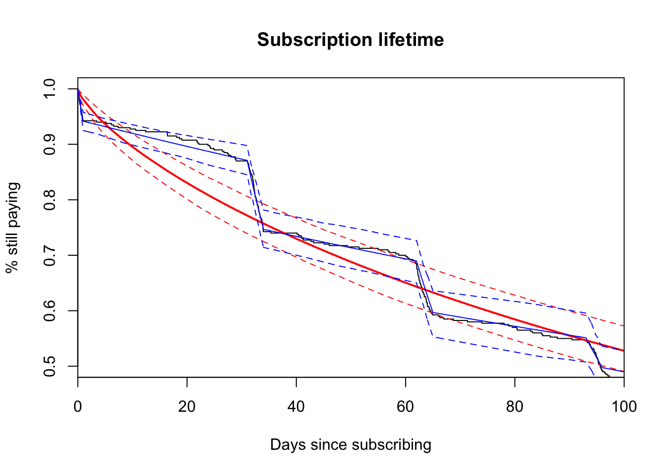
Very cool. Now we’re on our way to accurately measuring churn. The piecewise-constant model assumes a steady exponential rate between each interval. It is a parametric model. This isn’t a terrible assumption with real subscription data, though and it gives the problem tractibility. If you want to deploy an experiment that targets days 31 - 34 (when customers receive the first bill), using a parametric model will yield statistical power for a faster turnaround. Also, we can see that the generalized gamma distribution, a distribution that includes many other distributions, can’t cope with the quick drops caused by buyer’s remorse and bills. The piecewise-constant model yields a great fit for this type of data and can enable high-precision experiments.