Relationship of the Negative Binomial distribution and Poisson-Gamma mixture
rnbinom(10, 100, 0.5) %>%
  barplot(main = "Signups per day",
          ylab = "Signups",
          xlab = "Imaginary dates")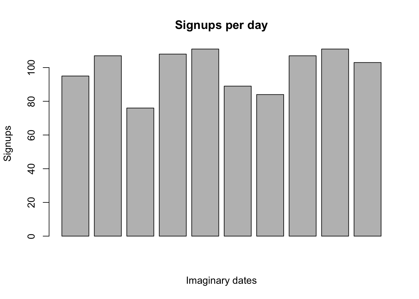
Many problems in SaaS analytics involve random arrival processes. It could be visits to landing pages, upgrades, churn, (insert your important event).
These are counting processes. If we’re lucky enough to have timestamps, we can measure the duration between events. The shorter the duration, the higher the count and vice versa.
The duration itself can be expected to change distribution parameters, or not. Homogenous Poisson point processes handle those of a constant rate, they’re the simple case. The duration might be stochastic and then we have a non-homogenous point process.
While I’ve been a student of the related theory and I’ve applied many MAS::glm.nb and pscl::zeroinfl models, I haven’t directly studied the relationship of the negative binomial and poisson-gamma mixture.
This document is incomplete. It’s a working document for my own study of these two ways of thinking about the same data: durations and counts.
# size = Gamma.shape
# prob = 1 / 1 + Gamma.scale
rnbinom(10000, size = 100, prob = 0.5) %>%
  hist(main = "Hist. Negative Binomial(r = 100, p = 0.5)")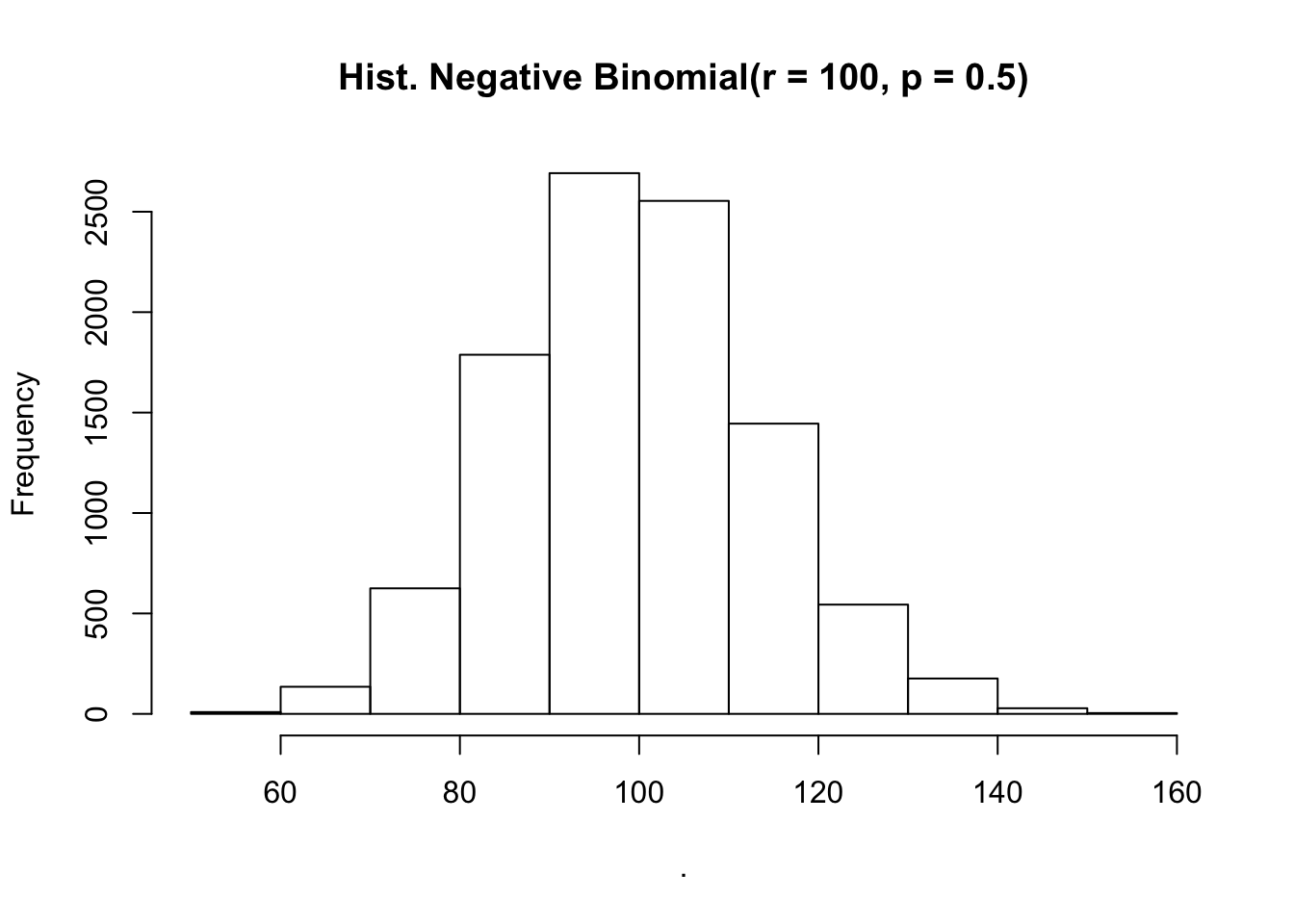
rgamma(n = 10000, shape = 100, scale = 1) %>%
  hist(main = "Hist. Gamma(shape = 100, scale = 1)")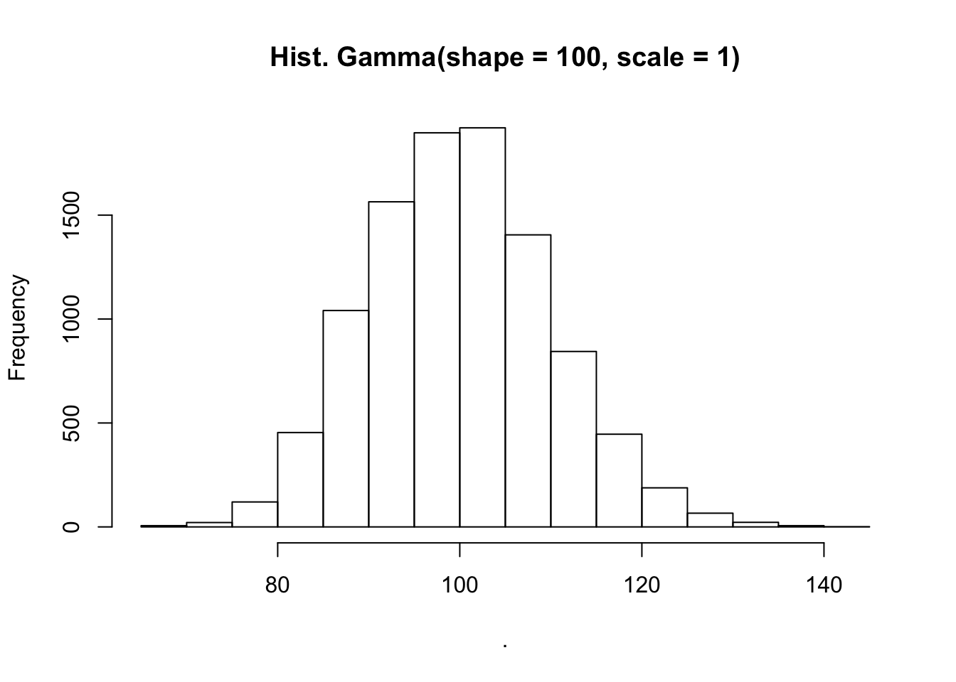
suppressPackageStartupMessages({library(purrr)})
seq_len(10000) %>%
  map_int(~ rpois(n = 1, lambda = rgamma(n = 1, shape = 100, scale = 1))) %>%
  hist(main = "Hist. Poisson(Gamma(shape = 100, scale = 1))")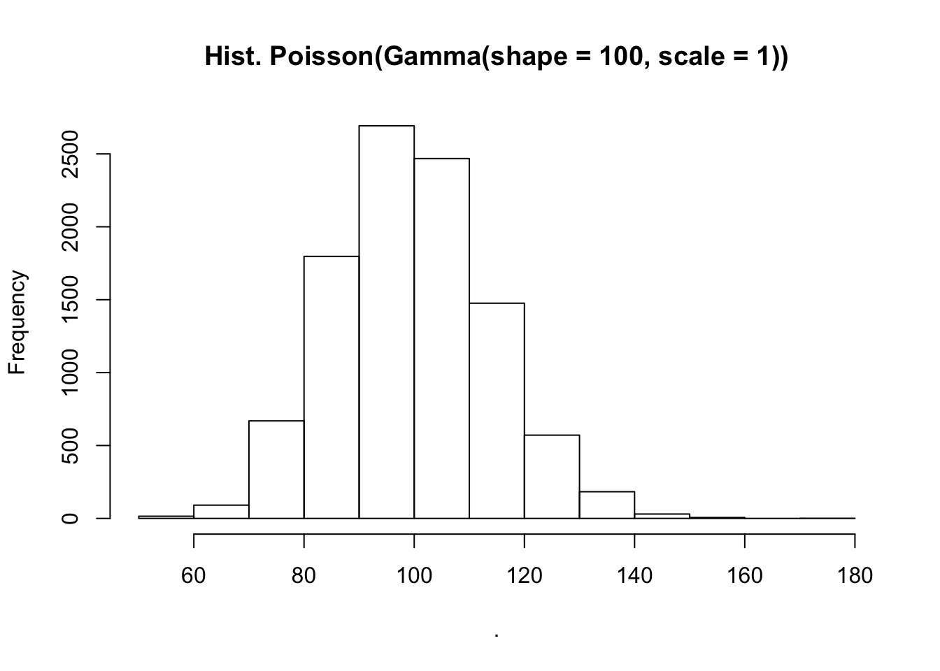
rnbinom(1e4, 100, 0.5) %>%
  hist(main = "Hist. NB(r = 100, p = 0.5)")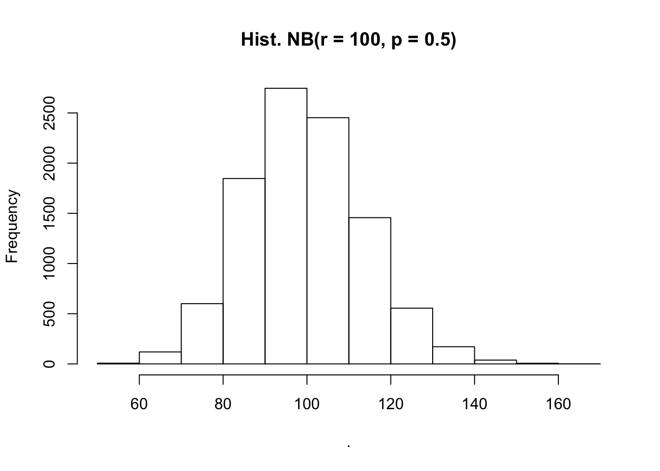
seq_len(1e4) %>%
  map_int(~ rpois(n = 1, lambda = rgamma(n = 1, shape = 100, scale = 1))) %>%
  ecdf() %>%
  plot(col = "red",
       main = "Empirical CDFs: rnbinom, rpois(rgamma)",
       xlim = c(120, 150), ylim = c(0.9, 1))

rnbinom(1e4, 100, 0.5) %>%
  ecdf() %>%
  plot(col = "blue", add = T)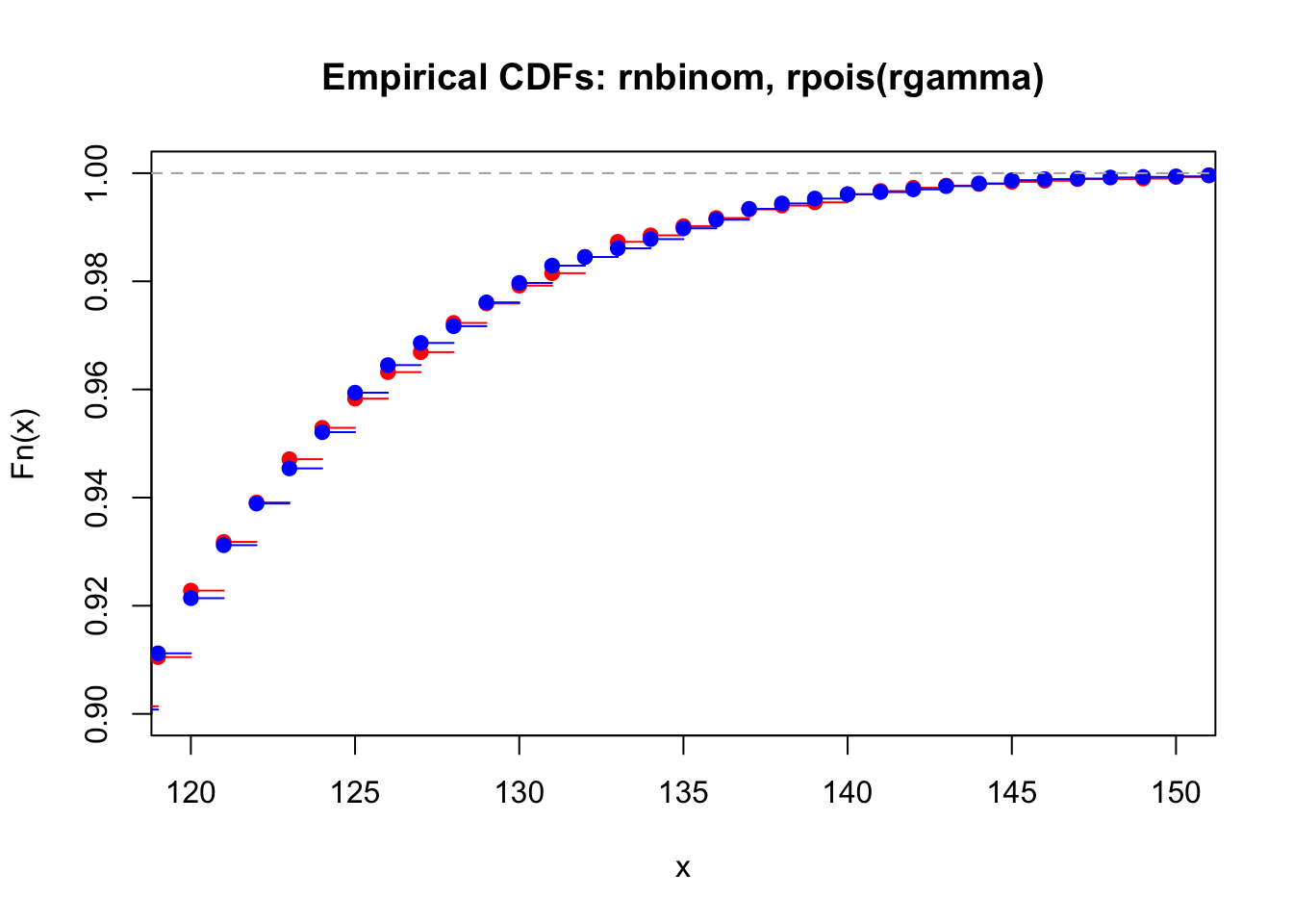
We can also directly inspect the distribution of the lambda parameter by reaching through negative binomial data and estimating the shape and rate (or scale) parameters of the Gamma distribution,
N <- 1e4
shape <- 0.5
rate <- 0.2
hist(lambdas <- rgamma(N, shape, rate = rate))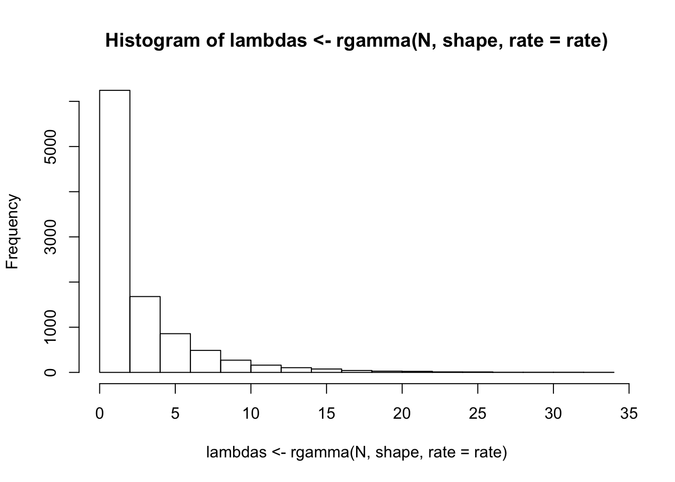
hist(x <- rpois(N, lambdas))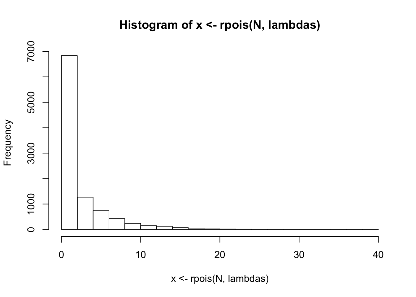
glm(x ~ 1, family = "poisson")##
## Call: glm(formula = x ~ 1, family = "poisson")
##
## Coefficients:
## (Intercept)
## 0.919
##
## Degrees of Freedom: 9999 Total (i.e. Null); 9999 Residual
## Null Deviance: 46000
## Residual Deviance: 46000 AIC: 63450# shape
MASS::glm.nb(x ~ 1)$theta## [1] 0.4864866# rate
MASS::glm.nb(x ~ 1)$theta/exp(coef(MASS::glm.nb(x ~ 1))[[1]])## [1] 0.194059