Benefit of introducing prior information in binomial experiments
The binomial distribution is such a handy tool. In this post I explore various ways to constuct confidence and credible intervals for binomial random variables.
Being a discrete distribution, the binomial distribution does not have an exact confidence interval. The discrete nature creates gaps and juts in the converage probability of any confidence interval placed on a binomial random variable proportion. The upshot is that your actual confidence level will not match the claimed confidence level. If you choose a 95% confidence interval but actually have an 85 or 90 percent confidence interval, the resulting intervals will not perform as expected. That is in practice you’ll find the proportion falling outside the interval more often than 95% of the time.
How can we fix the problem? A number of inventor-statisticians such as Abraham Wald, Alan Agresti and Brent A. Coull fix the problem with approximations of the exact confidence interval. I love the title of Agresti and Coull’s 1998 paper, “Approximate Is Better than “Exact” for Interval Estimation of Binomial Proportions”.
Another solution is to use a credible interval in place of a confidence interval. A credible interval is a probability statement than the true proportion falls within the interval and doesn’t suffer from the same coverage probability departure. I’m not yet exactly sure why credible intervals don’t suffer the same fate but I suspect it’s because the parameter is considered a random variable (continuous) rather than the data (discrete).
suppressPackageStartupMessages({
  library(dplyr)
  library(tibble)
  library(ggplot2)
  library(purrr)
  library(rstan)
  rstan_options(auto_write = TRUE)
})
organize_estimates <- function(x, interval_name) {
  # a little helper to organize all these intervals!
  x <- x %>% reduce(`-`) %>% abs()
  tibble(interval_width = x) %>%
    mutate(method = !!interval_name)
}
To start I’ll setup some constants. I’ll focus on a 95% interval length. I’ll also choose arbitrarily choose a sample size of 1,000 and “true known proportion” of 5 percent.
# Lets setup some constants for our simulation.
LOWER_INTERVAL <- 0.05/2
UPPER_INTERVAL <- 1 - (0.05/2)
SAMPLE_SIZE <- 1e3
TRUE_PROPORTION <- 0.05
Now I’ll simulate one instance of a binomial random variable with sample size 1k and true proportion 5 percent.
FAKE_DATA <- rbinom(1, size = SAMPLE_SIZE, prob = TRUE_PROPORTION)Now I’ll setup some functions that take in the FAKE_DATA (x) and SAMPLE_SIZE (N) and return an interval. The first interval I construct is via the so-called “Binomial exact test.” Of course there’s nothing exact about the test! However the test is also known by a different name: “[Binomial] Conservative Interval.” The promise of the test is that the confidence interval in practice will always achieve a confidence interval greater than the listed interval length. To say another way, if you ask for a 95% Conservative Interval you’ll get at least a 95% confidence level.
(fits <- binom.test(FAKE_DATA, SAMPLE_SIZE)$conf.int %>% organize_estimates("Conservative confidence interval"))## # A tibble: 1 x 2
## interval_width method
## <dbl> <chr>
## 1 0.02880593 Conservative confidence intervalNext I’ll write a function that leverages the fact the beta distribution is a conjugate prior for the binomial distribution. The function takes in the fake data and prior information and returns a 95% credible interval.
conjugate_bayesian_ci <- function(prior, x, N) {
  qbeta(p = c(LOWER_INTERVAL, UPPER_INTERVAL), shape1 = prior[[1]] + x, shape2 = prior[[2]] + N - x)
}
conjugate_bayesian_ci(prior = c(50, 950), FAKE_DATA, SAMPLE_SIZE)
## [1] 0.04224873 0.06160038fits <- fits %>%
bind_rows(conjugate_bayesian_ci(prior = c(5, 95), FAKE_DATA, SAMPLE_SIZE) %>% organize_estimates("Simple Bayes w/ 5, 95 prior")) %>%
bind_rows(conjugate_bayesian_ci(prior = c(50, 950), FAKE_DATA, SAMPLE_SIZE) %>% organize_estimates("Simple Bayes w/ 50, 950 prior"))I’ve been using stan a good bit lately to learn and practice Bayesian statistics. Markov chain monte carlo is really computationally expensive realtive to the conjugate prior-leveraging method, so I add it here as stan practice rather than as an improvement on the conjugate method for this problem. Similar to conjugate_bayeisna_ci, mcmc_bayesian_ci takes in prior information and data and returns a credible interval.
mcmc_bayesian_ci <- function(prior, x, N) {
  if(missing(x) | missing(N)) {
    x <- x; n <- N;
  }
  # prior <- 'p ~ beta(10, 90);'
  model_code <- glue::glue('
  data {{
    int x;
    int trials;
  }}
  parameters {{
    real p;
  }}
  model {{
    { prior }
    x ~ binomial(trials, p);
  }}
  ')
  method_name <- glue::glue("Bayes w/ prior { prior }")
  sink("file")
  x <- rstan::stan(
    model_code = model_code,
    model_name = "anon_model",
    data = list(
      x = x, trials = N
    ),
    refresh = 0) %>%
    rstan::extract("p") %>% pluck("p") %>% quantile(c(LOWER_INTERVAL, UPPER_INTERVAL)) %>%
    organize_estimates(method_name)
  sink()
  return(x)
}
fits <- fits %>%
bind_rows(mcmc_bayesian_ci(FAKE_DATA, SAMPLE_SIZE, prior = "p ~ beta(5, 95);")) %>%
bind_rows(mcmc_bayesian_ci(FAKE_DATA, SAMPLE_SIZE, prior = "p ~ beta(50, 950);")) %>%
bind_rows(mcmc_bayesian_ci(FAKE_DATA, SAMPLE_SIZE, prior = "p ~ uniform(0, 1);"))Here are our interval widths so far,
fits %>% arrange(desc(interval_width)) %>% mutate_if(is.numeric, scales::percent)## # A tibble: 6 x 2
## interval_width method
## <chr> <chr>
## 1 2.535% Conservative confidence interval
## 2 2.421% Bayes w/ prior p ~ uniform(0, 1);
## 3 2.369% Bayes w/ prior p ~ beta(5, 95);
## 4 2.336% Simple Bayes w/ 5, 95 prior
## 5 1.815% Simple Bayes w/ 50, 950 prior
## 6 1.804% Bayes w/ prior p ~ beta(50, 950);While I appreciate that binom.test is the conservative interval behind the scenes, I wanted to double-check for myself hence conservative_interval2 below. I also add the three main Frequentist approximations: Jefferys, Wald, and Agresti-Coull.
conservative_interval2 <- function(x, n) {
  c(qbeta(LOWER_INTERVAL, x, n - x + 1), qbeta(UPPER_INTERVAL, x + 1, n - x))
}

wald_ci <- function(x, n) {
  p_hat <- x / n
  wald_factor <- qnorm(UPPER_INTERVAL)*sqrt(p_hat * (1 - p_hat) / n)
  c(
    p_hat - wald_factor,
    p_hat + wald_factor
  )
}

agresti_coull_ci <- function(x, n) {
  wald_ci(x + 2, n + 4)
}

jefferys_ci <- function(x, n) {
  c(qbeta(LOWER_INTERVAL, x + 0.5, n - x + 0.5), qbeta(UPPER_INTERVAL, x + 0.5, n - x + 0.5))
}conservative_interval2(FAKE_DATA, SAMPLE_SIZE) %>% organize_estimates("Conservative interval2") %>%
bind_rows(fits) %>%
bind_rows(wald_ci(FAKE_DATA, SAMPLE_SIZE) %>% organize_estimates("Wald interval")) %>%
bind_rows(agresti_coull_ci(FAKE_DATA, SAMPLE_SIZE) %>% organize_estimates("Agresti-Coull interval")) %>%
bind_rows(jefferys_ci(FAKE_DATA, SAMPLE_SIZE) %>% organize_estimates("Jefferys interval")) %>%
arrange(desc(interval_width)) %>%
mutate(method = factor(method, levels = unique(method))) %>%
ggplot(aes(x = method, y = interval_width)) +
geom_bar(stat = "identity", colour = "black") +
coord_flip() +
scale_y_continuous(breaks = scales::pretty_breaks(10), labels = scales::percent) +
xlab("Method") +
ylab("Interval width (around 5%)") +
ggtitle("Interval widths for our FAKE_DATA\n(known 5% proportion, 1k samples)")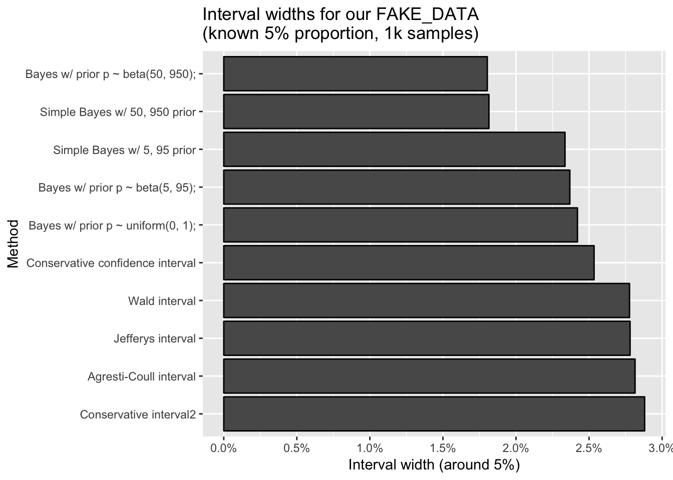
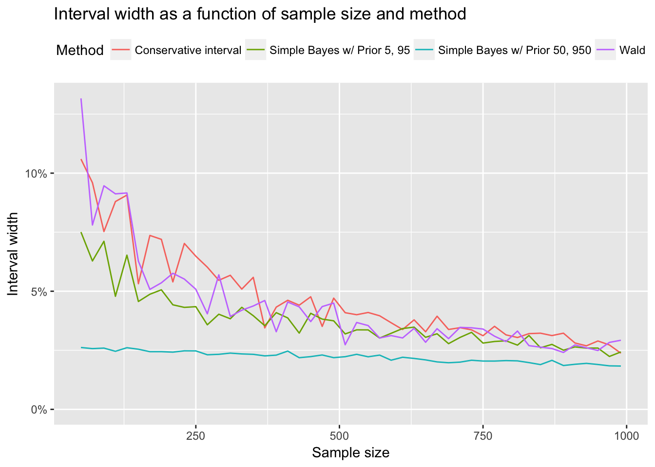
Finally as a small bonus, I wanted to get a rough view of how quickly the Bayesian credible intervals and Wald converge as sample size grows.
fit_wald <- function(p, N) {
  rbinom(1, size = N, prob = p) %>%
    wald_ci(N) %>%
    reduce(`-`) %>%
    abs() %>%
    as_tibble() %>%
    mutate(N = !!N, method = "Wald") %>%
    select(N, interval_width = value, method)
}
fit_conservative <- function(p, N) {
  rbinom(1, size = N, prob = p) %>%
    conservative_interval2(N) %>%
    reduce(`-`) %>%
    abs() %>%
    as_tibble() %>%
    mutate(N = !!N, method = "Conservative interval") %>%
    select(N, interval_width = value, method)
}
fit_bayes <- function(p, N, prior) {
  x <-  rbinom(1, size = N, prob = p)
  method <- glue::glue("Simple Bayes w/ Prior { prior[[1]] }, { prior[[2]] }")
  conjugate_bayesian_ci(prior, x = x, N = N) %>%
    organize_estimates(method) %>%
    mutate(N = !!N) %>%
    select(N, interval_width, method)
}

SAMPLE_SIZES <- seq(50, 1e3, 20)

apply_fit <- function(f) {
  SAMPLE_SIZES %>%
    map(~ f(TRUE_PROPORTION, .x)) %>%
    bind_rows()
}
apply_bayes <- function(f, prior) {
  SAMPLE_SIZES %>%
    map(~ f(TRUE_PROPORTION, .x, prior)) %>%
    bind_rows()
}

apply_fit(fit_wald) %>%
  bind_rows(apply_fit(fit_conservative)) %>%
  bind_rows(apply_bayes(fit_bayes, prior = c(5, 95))) %>%
  bind_rows(apply_bayes(fit_bayes, prior = c(50, 950))) %>%
  ggplot(aes(x = N, y = interval_width, colour = factor(method))) +
  geom_line() +
  # geom_smooth(method = "gam", formula = y ~ s(x, bs = "ps")) +
  expand_limits(y = 0) +
  scale_y_continuous(labels = scales::percent) +
  scale_color_discrete(name = "Method") +
  theme(legend.position = "top") +
  ylab("Interval width") +
  xlab("Sample size") +
  ggtitle("Interval width as a function of sample size and method")