Is Airbus Safer Than Boeing?
Based on this analysis of NTSB event data normalized by flight departures, Boeing appears to have approximately 1.7× more safety events per 100,000 departures than Airbus. This gap is not a recent spike driven by media attention; it has persisted for over a decade in the data examined here. That said, a single analysis is not conclusive, and both manufacturers are extremely safe — flying is roughly 100× safer than driving, and in most years zero people die in US commercial plane crashes.
| Metric | Boeing | Airbus |
|---|---|---|
| NTSB events per 100k departures | 6.5 | 3.8 |
| Relative rate | 1.7× | 1.0× (baseline) |
| Trend | Persistent gap | Consistently lower |
| Stock performance (2019–2024) | −49% | +42% |
Background
Boeing has been in the news a lot recently for all kinds of apparent malfunctions and issues. Last night, I noticed Joe Weisenthal ask whether this represented a real problem or confirmation bias (as can happen when our collective attention is newly trained on an issue). I wondered the same thing, and before this analysis I was unsure whether Boeing or Airbus are safer. So I decided to collect some data and check for myself.
Before I begin, it's important to note that traveling by airplane is far safer than driving (and that's extremely hard to understate). In most years zero people die in commercial plane crashes in the US whereas tens of thousands die in car crashes per year in the US (~ about 40k). I would much rather fly on either Boeing or Airbus cross-country than drive from a safety perspective (it's not even close and I wouldn't think twice about flying Boeing tomorrow vs. driving). That said, I am curious about which airplane maker I should prefer from a safety perspective.
Data & Methodology
To compare Boeing and Airbus's records, I used NTSB event data from data.ntsb.gov. Boeing flies more flights than Airbus in the US, so it's important to normalize — we'd typically expect more events from a more popular maker. I downloaded flight departure data from the Department of Transportation and calculated NTSB events per 100,000 departures.
library(tidyverse)
library(mdbr)

read_mdb("boeing-analysis/avall.mdb", "events") -> events
read_mdb("boeing-analysis/avall.mdb", "aircraft") -> aircraft

events %>%
  mutate(date = as.POSIXct(ev_date, format = "%m/%d/%y %H:%M:%S", tz = "UTC")) %>%
  left_join(aircraft, by = "ev_id") %>%
  distinct(ev_id, Aircraft_Key, .keep_all = T) -> d

# Count events by make and half-year
d %>%
  count(acft_make,
        accident_date = lubridate::floor_date(date, "half")) %>%
  group_by(acft_make) %>%
  complete(accident_date = seq.POSIXt(min(accident_date), max(accident_date), by = "6 month"),
           fill = list(n = 0)) %>%
  mutate(n_minus_avg = n - mean(n)) %>%
  ungroup() -> events_by_make
Boeing vs Airbus: Which Is Safer?
The result indicates that Boeing has more NTSB events per departure, about 6.5 per 100k departures vs. 3.8 per 100k for Airbus. That's about 1.7x more events per departure than Airbus.
events_by_make2 %>%
  ggplot(aes(date, events_per_100k_departures, color = factor(type))) +
  geom_line(linewidth = 1) +
  geom_point(size = 3) +
  geom_hline(yintercept = 0) +
  ggthemes::scale_color_colorblind(name = "") +
  theme_bw(20) +
  scale_x_datetime(date_breaks = "1 year", date_labels = "%Y") +
  ylab("NTSB events per 100k departures") +
  ggtitle("NTSB events per 100k departures") +
  xlab("Year")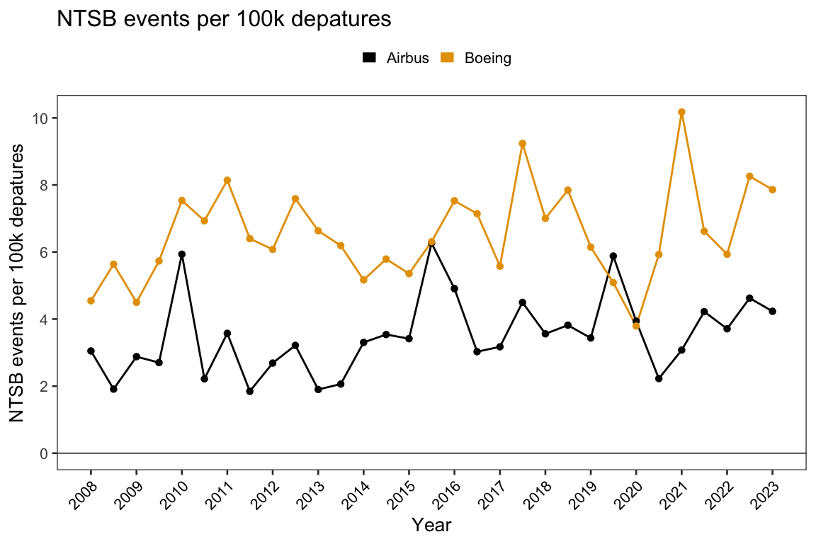
That Airbus has fewer incidents than Boeing isn't that surprising to me given the news. Also, I notice that Boeing's advertisement for "reliability engineers" doesn't require that those engineers have a degree in statistics. In my mind, if you're hiring people whose responsibility it is to perform statistical analysis in important situations, it's best to hire statisticians with degrees in statistics.

Boeing's stock value has significantly under-performed Airbus from 2019 to March 2024, a 49% decline vs. 42% growth, respectively.

Linear Model
# Assume 0 events given 0 departures by not including an intercept
lm(events ~ I(departures_performed / 1e5) : type - 1,
   data = events_by_make2) -> fit

summary(fit)
## Coefficients:
##                                          Estimate Std. Error t value Pr(>|t|)
## I(departures_performed/1e+05):typeAirbus   3.7716     0.3889   9.698 6.73e-14 ***
## I(departures_performed/1e+05):typeBoeing   6.5120     0.1862  34.968  < 2e-16 ***
Conclusion
This is clearly a long-term issue, not a recent one. To address Joe's original question: standing back, I'd say this falls more into the shark attack / confirmation bias camp (as opposed to representing a significant near-term uptick). Still, it is concerning that Boeing has persistently more events per departure than Airbus.
That said, I still wouldn't be concerned about flying in a plane produced by either company. Air travel remains one of the safest modes of transportation available. The rigorous testing, maintenance, and oversight that aircraft from reputable manufacturers undergo are unparalleled. While it's wise to be aware of the risks, letting fear of flying limit your opportunities is to ignore the overwhelming evidence of its safety.
Related Statistical Methods
- 📊 Simulating Right-Censored Weibull Data — Survival analysis techniques used in reliability engineering
- 📐 Why Is the Characteristic Life 63.2%? — The mathematical constant behind failure analysis
- 🎲 Poisson-Gamma Negative Binomial — Count-based event modeling used in safety analysis