Geometric Distribution and Bayesian Updating

The concept of Bayesian updating is fascinating: encode information using a likelihood and readily update the likelihood with each subsequent data point. The prior (what we believe encoded from previous observation) and the likelihood (our "story") are an engine for producing posterior distributions.

Certain distributions have conjugate priors — distributions whose likelihood functions are proportional to each other, constants aside. Using conjugacy enables very computationally cheap updating, in contrast to Markov Chain Monte Carlo methods.

Counting Distributions and the Beta Conjugate

The counting distributions — Bernoulli, Binomial, Geometric, and Negative Binomial — all share the Beta distribution as their conjugate prior. This means we can directly update a Beta distribution having observed a heads/tails type process.

Setting Up the Process

Below I define a coin-flip process with a probability of heads on any given flip of 5 percent. I encode a weak, uninformative prior belief:

set.seed(0)
magical_unknown_param <- 0.05
original_belief_a <- 1
original_belief_b <- 1

First Observation

Draw one observation from a geometric distribution by flipping the coin until we see the first heads. The result is the number of tails along the way:

(x <- rgeom(1, prob = magical_unknown_param))
## [1] 4

It took four tails in a row before we observed the first heads. Let's update our beliefs:

updated_belief_a <- original_belief_a + 1
updated_belief_b <- original_belief_b + sum(x)
(updated_beliefs <- rbeta(1, updated_belief_a, updated_belief_b))
## [1] 0.6236603

Sequential Updating

Now repeat the process, accumulating observations and updating beliefs each time:

# Second observation
(x <- c(x, rgeom(1, prob = magical_unknown_param)))
## [1]  4 10

(updated_belief_a <- original_belief_a + 1)
## [1] 2
(updated_belief_b <- original_belief_b + sum(x))
## [1] 15
(updated_beliefs <- rbeta(1, updated_belief_a, updated_belief_b))
## [1] 0.02604405

# Third observation
(x <- c(x, rgeom(1, prob = magical_unknown_param)))
## [1]  4 10 37

(updated_belief_b <- original_belief_b + sum(x))
## [1] 52
(updated_beliefs <- rbeta(1, updated_belief_a, updated_belief_b))
## [1] 0.07199219

# Fourth observation
(x <- c(x, rgeom(1, prob = magical_unknown_param)))
## [1]  4 10 37 16

(updated_belief_b <- original_belief_b + sum(x))
## [1] 68
(updated_beliefs <- rbeta(1, updated_belief_a, updated_belief_b))
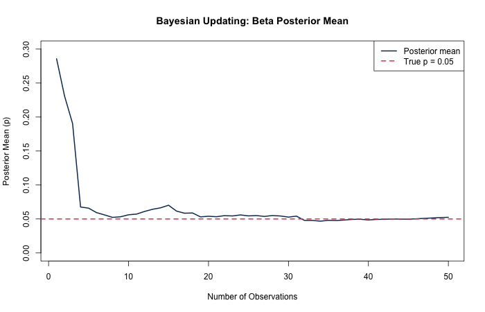
## [1] 0.02166169

Visualizing the convergence of the posterior mean across many observations: