Ordinary least squares in stan
I’m just getting up to speed with stan. The sheer number of ways stan can be used (probabilistic programming) makes it tempting to try and build complex models right way. I’m going to avoid that temptation and start with one of the simplest models I know, ordinary least squares,
\(y = XB + \epsilon\)
library(rstan)
library(purrr)
library(dplyr)
library(ggplot2)
rstan_options(auto_write = TRUE)
options(mc.cores = parallel::detectCores())
First, I’ll generate some ols data with pretend “true” parameter values,
set.seed(1)
N <- 80
x <- runif(N)
intercept <- 5
slope <- 3
y <- intercept + x * slope + rnorm(N)
\(y = 5 + 3 \times X + \epsilon\) where \(\epsilon \sim N\)
plot(x, y, main = "A scatterplot")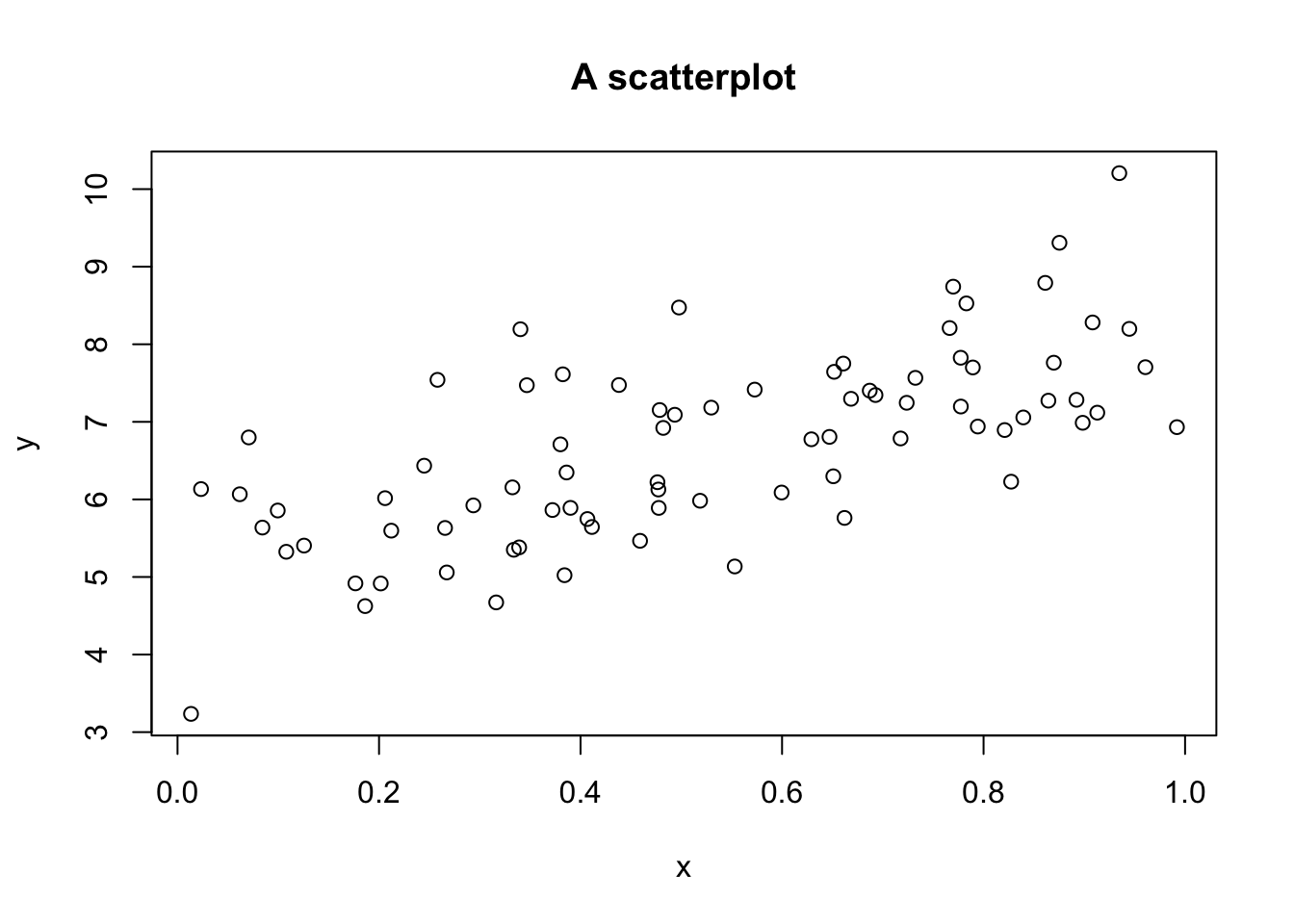
Now let’s check that I didn’t make a mistake generating the data,
summary(lm(y ~ x))##
## Call:
## lm(formula = y ~ x)
##
## Residuals:
## Min 1Q Median 3Q Max
## -1.91345 -0.69202 -0.07729 0.51178 2.27503
##
## Coefficients:
## Estimate Std. Error t value Pr(>|t|)
## (Intercept) 5.1082 0.2193 23.298 < 2e-16 ***
## x 3.0196 0.3716 8.125 5.38e-12 ***
## ---
## Signif. codes: 0 '***' 0.001 '**' 0.01 '*' 0.05 '.' 0.1 ' ' 1
##
## Residual standard error: 0.89 on 78 degrees of freedom
## Multiple R-squared: 0.4584, Adjusted R-squared: 0.4515
## F-statistic: 66.02 on 1 and 78 DF, p-value: 5.382e-12This looks like I’d expect with an intercept close to 5 and a slope close to 3.
model_code <- "
data {
  int N;
  vector[N] x; // covariate
  vector[N] y; // outcomes
}
parameters {
  real intercept;
  real slope;
  real<lower=0> sigma;
}
model {
  intercept ~ normal(0, 5);
  slope ~ normal(0, 5);

  y ~ normal(intercept + slope * x, sigma);
}"
(estimates <- extract(fit, pars = c("intercept", "slope"))) %>% map(mean)## $intercept
## [1] 5.106859
##
## $slope
## [1] 3.017778capitalize <- function(x) { paste0(toupper(substr(x, 1, 1)), substr(x, 2, nchar(x))) }
theme_especial <- function() {
theme_bw() + theme(strip.text = element_text(colour = "black"),
axis.text = element_text(colour = "black"))
}
as_tibble(estimates) %>%
reshape2::melt() %>%
mutate(true_value = ifelse(variable == "intercept", intercept, slope)) %>%
mutate(variable = capitalize(as.character(variable))) %>%
ggplot(aes(x = value)) +
geom_histogram(colour = "black", binwidth = 0.1) +
geom_vline(aes(xintercept = true_value), color = "red") +
facet_wrap(~ variable, scales = "free") +
ggtitle("Parameter estimates vs. actual true values") +
xlab("") + theme_especial()## No id variables; using all as measure variables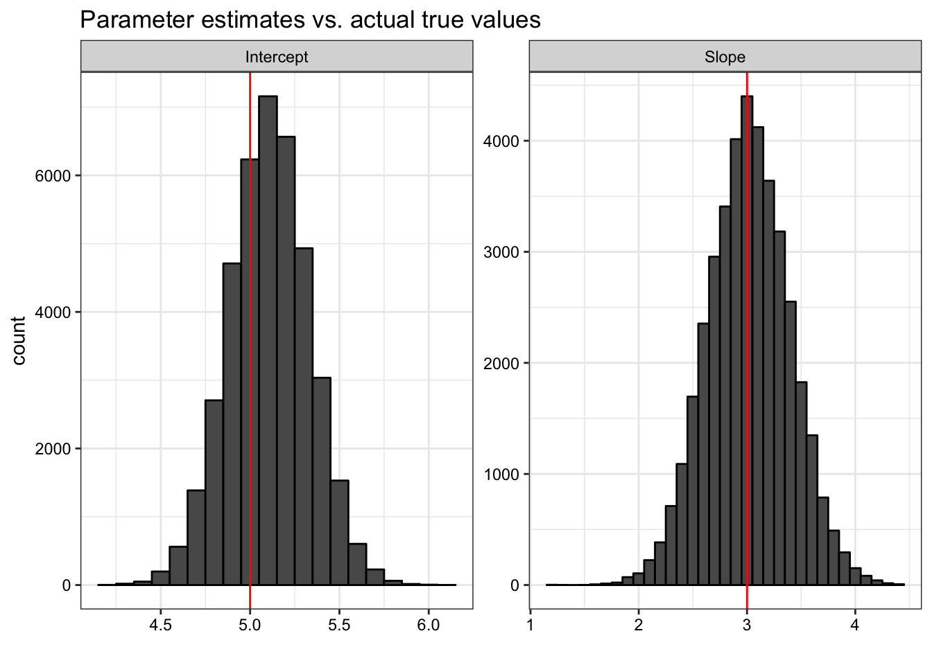
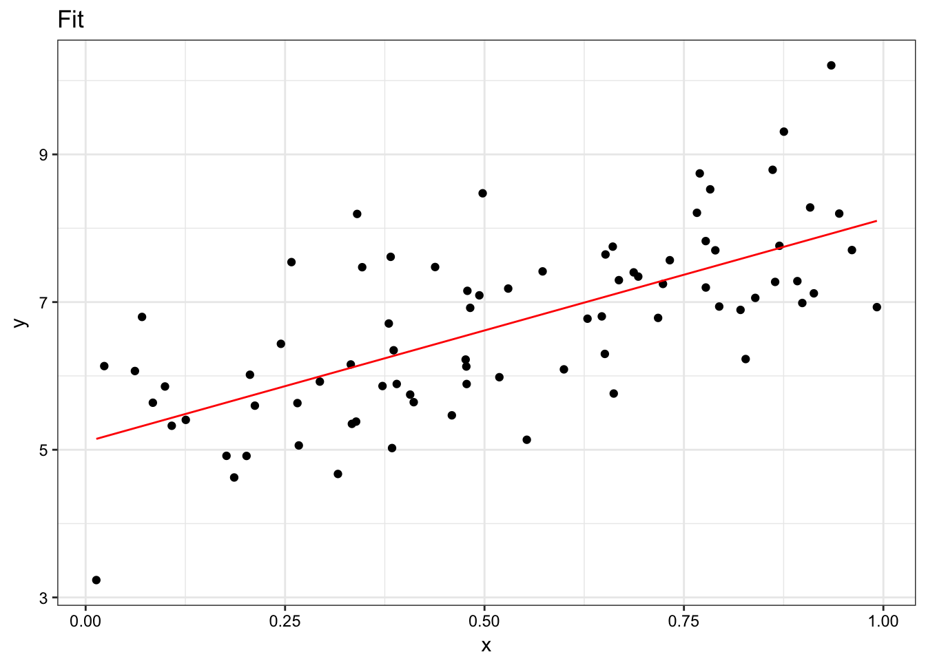
tibble(y = y, x = x) %>%
  mutate(model = mean(estimates$intercept) + mean(estimates$slope) * x) %>%
  ggplot(aes(x = x, y = y)) +
  geom_point() +
  geom_line(aes(y = model), colour = "red") +
  ggtitle("Fit") +
  theme_especial()