What Is the Poisson-Gamma Mixture?
The Negative Binomial distribution is mathematically equivalent to a Poisson distribution whose rate parameter \(\lambda\) is itself drawn from a Gamma distribution. If \(\lambda \sim \text{Gamma}(r, \beta)\) and \(X \mid \lambda \sim \text{Poisson}(\lambda)\), then the marginal distribution of \(X\) is Negative Binomial with parameters \(r\) and \(p = 1/(1 + \beta)\).
This equivalence is why the NB is the standard model for overdispersed count data — it naturally handles heterogeneity in rates across individuals, which a plain Poisson cannot.
Why This Matters in Practice
Many problems in SaaS analytics involve random arrival processes. It could be visits to landing pages, upgrades, churn — insert your important event. These are counting processes. If we're lucky enough to have timestamps, we can measure the duration between events. The shorter the duration, the higher the count and vice versa.
The duration itself can be expected to change distribution parameters, or not. Homogeneous Poisson point processes handle those of a constant rate — they're the simple case. The duration might be stochastic and then we have a non-homogeneous point process.
While I've applied many MASS::glm.nb and pscl::zeroinfl models,
I wanted to directly study the relationship between the negative binomial and the Poisson-Gamma
mixture. This document explores that equivalence through simulation.
Simulating Negative Binomial Counts
rnbinom(10, 100, 0.5) %>%
  barplot(main = "Signups per day",
          ylab = "Signups",
          xlab = "Imaginary dates")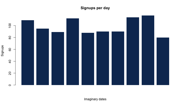
Comparing the Distributions Side by Side
The key insight is that a Negative Binomial random variable can be equivalently generated as a Poisson random variable whose rate parameter is itself drawn from a Gamma distribution.
# Negative Binomial directly
# size = Gamma.shape
# prob = 1 / (1 + Gamma.scale)
rnbinom(10000, size = 100, prob = 0.5) %>%
hist(main = "Hist. Negative Binomial(r = 100, p = 0.5)")
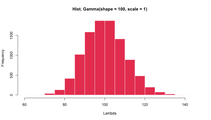
# Gamma distribution of rates
rgamma(n = 10000, shape = 100, scale = 1) %>%
hist(main = "Hist. Gamma(shape = 100, scale = 1)")
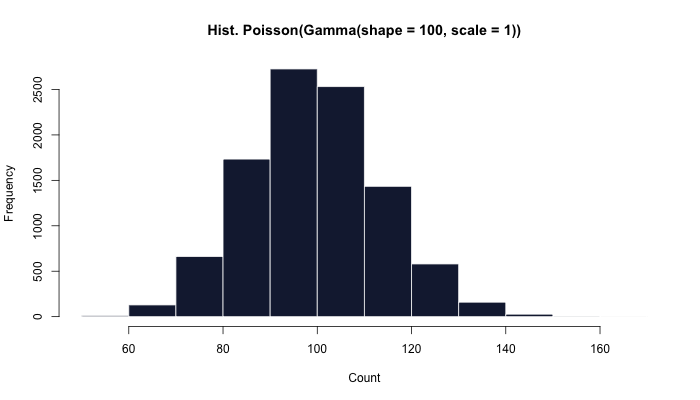
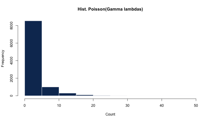
# Poisson-Gamma mixture (equivalent to Negative Binomial)
suppressPackageStartupMessages({library(purrr)})
seq_len(10000) %>%
map_int(~ rpois(n = 1,
lambda = rgamma(n = 1, shape = 100, scale = 1))) %>%
hist(main = "Hist. Poisson(Gamma(shape = 100, scale = 1))")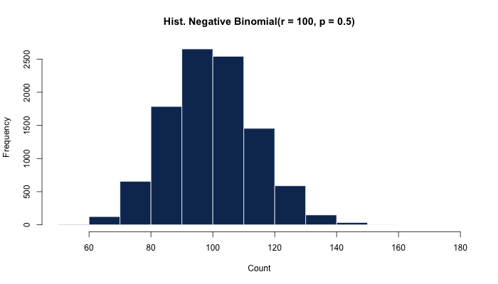
Empirical CDF Comparison
To verify the equivalence, we overlay the empirical CDFs of both approaches:
seq_len(1e4) %>%
  map_int(~ rpois(n = 1,
    lambda = rgamma(n = 1, shape = 100, scale = 1))) %>%
  ecdf() %>%
  plot(col = "red",
       main = "Empirical CDFs: rnbinom vs rpois(rgamma)",
       xlim = c(120, 150), ylim = c(0.9, 1))
rnbinom(1e4, 100, 0.5) %>%
  ecdf() %>%
  plot(col = "blue", add = TRUE)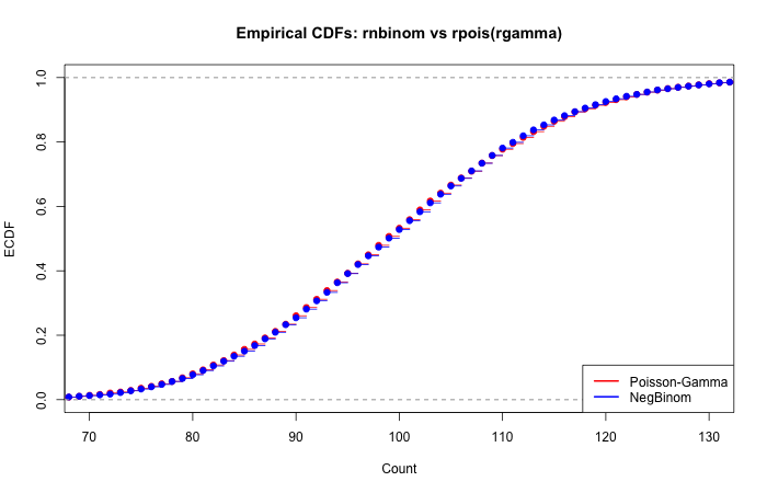
The CDFs overlap almost perfectly, confirming the distributional equivalence.
Recovering the Gamma Parameters
We can directly inspect the distribution of the λ parameter by reaching through negative binomial data and estimating the shape and rate parameters of the underlying Gamma distribution:
N <- 1e4
shape <- 0.5
rate <- 0.2
hist(lambdas <- rgamma(N, shape, rate = rate))
hist(x <- rpois(N, lambdas))

# Poisson GLM (ignoring overdispersion)
glm(x ~ 1, family = "poisson")

# Negative binomial recovers the Gamma shape
# shape
MASS::glm.nb(x ~ 1)$theta
## [1] 0.4864866

# rate
MASS::glm.nb(x ~ 1)$theta /
  exp(coef(MASS::glm.nb(x ~ 1))[[1]])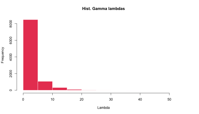
Related Statistical Methods
- 📊 Bernoulli Experiments & Stan MCMC — Building likelihood functions from scratch
- 📐 Why Is the Characteristic Life 63.2%? — The Weibull distribution's connection to Euler's number
- ✈️ Boeing vs Airbus Safety Analysis — NTSB event data analysis using count models