How and why Poisson regression
Count data are ubiquitous, but the methods to analyze them aren’t as well-known. In this tutorial, you’ll learn a basic method for improving on least squares when analyzing counts.
You may be thinking, can’t I just use least squares? Sure, but then you shouldn’t be surprised if the model predicts “negative counts.” Let’s take a look at a quick example.
First, I’ll simulate some data,
set.seed(0)
N <- 20 # days of data
intercept <- 10
slope <- -0.5
days <- seq_len(N)

widgets <- rpois(N, lambda = intercept + slope * days)

(data.frame(days = days, widgets = widgets) -> d)
# install.packages("ggplot2") # uncomment and run first
library(ggplot2)
ggplot(d, aes(x = days, y = widgets)) +
geom_bar(stat = "identity") +
labs(x = "Ficticious days", y = "Widgets", title = "Counts to analyze")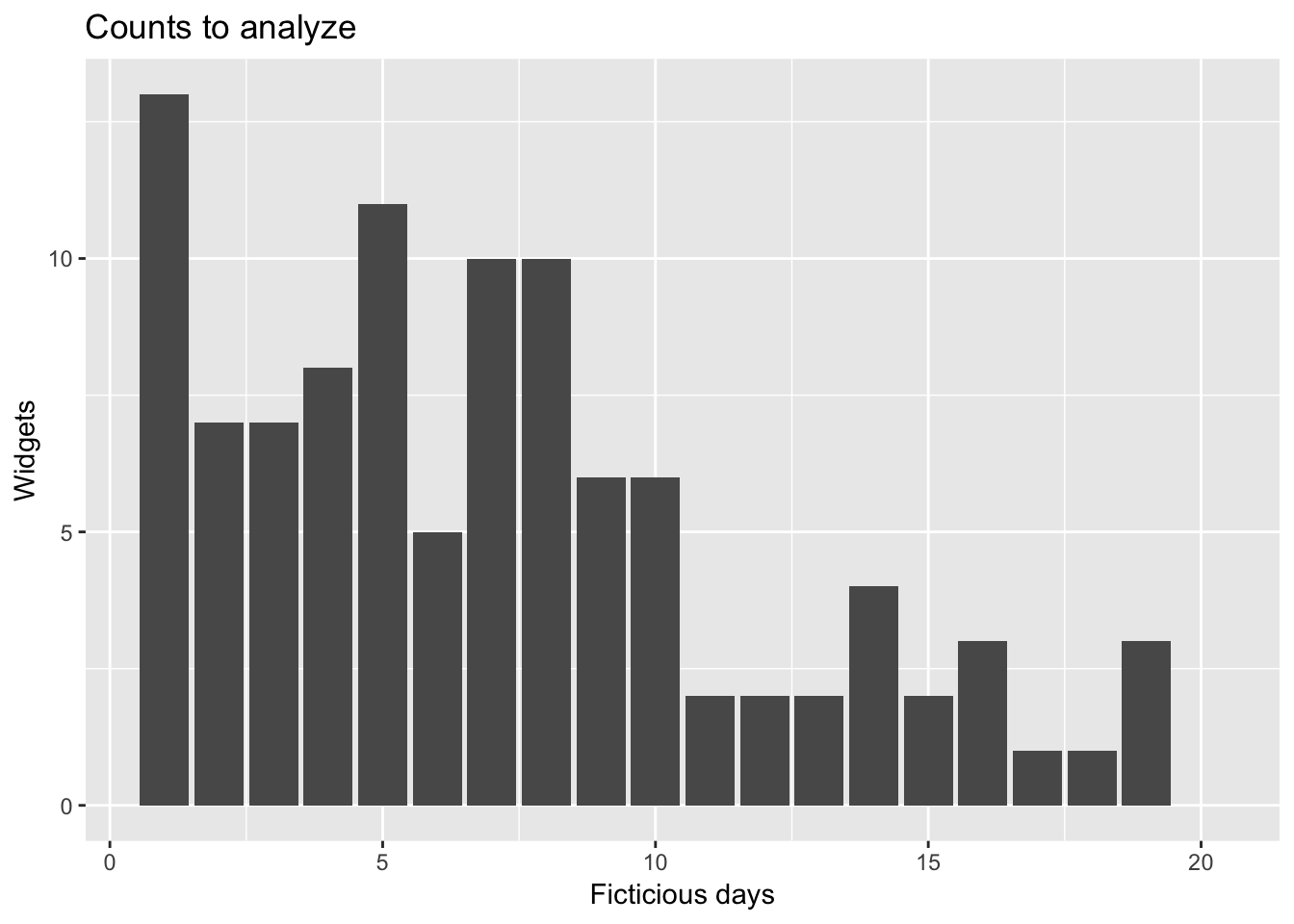
Now, let’s fit a least squares line,
(lm(widgets ~ days, data = d) -> fit)##
## Call:
## lm(formula = widgets ~ days, data = d)
##
## Coefficients:
## (Intercept) days
## 10.7474 -0.5331Next, let’s see how our model fits,
# install.packages("dplyr") # uncomment and run first
suppressPackageStartupMessages(library(dplyr))
d %>%
  mutate(estimated_counts = predict(fit, newdata = ., type = "response")) %>%
  ggplot(aes(x = days)) +
  geom_bar(aes(y = widgets), stat = "identity") +
  geom_line(aes(y = estimated_counts), colour = "red") +
  geom_point(aes(y = estimated_counts), colour = "red") +
  labs(y = "Widgets", x = "Days") +
  NULL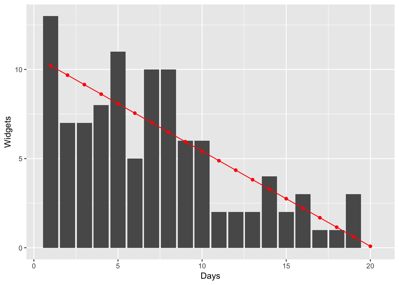
If we extrapolate a bit, we can see that negative counts will be predicted,
predict_widgets <- function(model) {
  d %>%
    bind_rows(data.frame(days = seq(21, 25, 1), widgets = NA)) %>%
    mutate(estimated_counts = predict(model, newdata = ., type = "response")) %>%
    ggplot(aes(x = days)) +
    geom_bar(aes(y = widgets), stat = "identity") +
    geom_line(aes(y = estimated_counts), colour = "red") +
    geom_point(aes(y = estimated_counts), colour = "red") +
    labs(y = "Widgets", x = "Days") +
    NULL
}
predict_widgets(fit)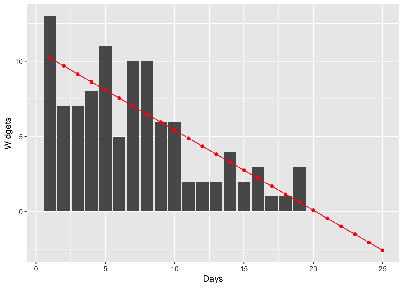
Poisson regression solves this problem by adding the assumption, “the response variable must be >= 0.” Now let’s re-analyze the same data using Poisson regression.
(glm(widgets ~ days, data = d, family = "poisson") -> pfit)##
## Call: glm(formula = widgets ~ days, family = "poisson", data = d)
##
## Coefficients:
## (Intercept) days
## 2.6137 -0.1119
##
## Degrees of Freedom: 19 Total (i.e. Null); 18 Residual
## Null Deviance: 56.13
## Residual Deviance: 18.01 AIC: 85.05suppressPackageStartupMessages(library(dplyr))
predict_widgets(pfit)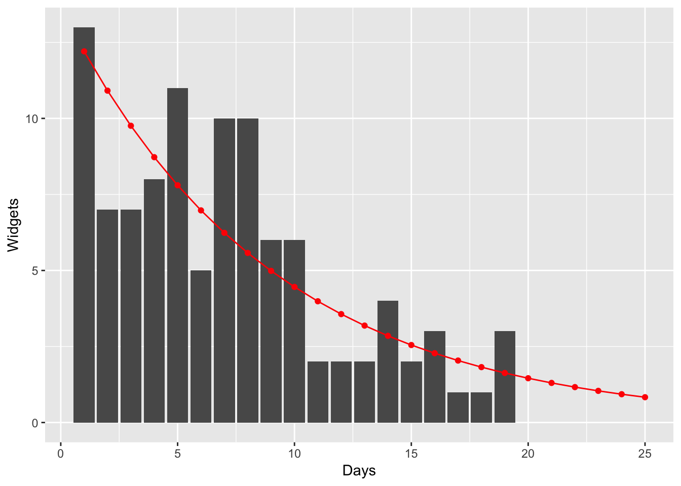
Tada! So how does it work? Poisson regression works similarly to least squares, except first the method transforms the data using the log function before estimating the intercept and slope parameters. Then in the fitting step, instead of using the model widgets = intercept + slope * days, the formula is widgets = exp(intercept + slope * days). The exp function isn’t defined below 0. Voila! Poisson regression will never predict negative counts!
You might think, “well, business is great, we’re selling more widgets every day, do I need Poisson regression?” Probably not, you can probably get away with least squares just fine. However if your company has many many product lines, it might be difficult to inspect each application of the model. In this case, it’s possible to use Poisson regression to avoid an embarassing situation of having to explain the rare case of predictions below 0. If that occurs, stakeholders might come to doubt the model overall. Since using Poisson regression is so cheap relative to least squares, why not protect yourself from that situation?
Thanks for reading!