Real-time experiments
Suppose we’d like to follow along as our experiment runs. However we’re worried about the effect of applying a stopping rule to our experiment. One thing we could do is apply a well calibrated prior to counter-act the act of peeking.
rbeta(1e3, 1e3*0.1, 1e3*0.9) %>% hist(main = "Prior", xlab = "Conversion rate")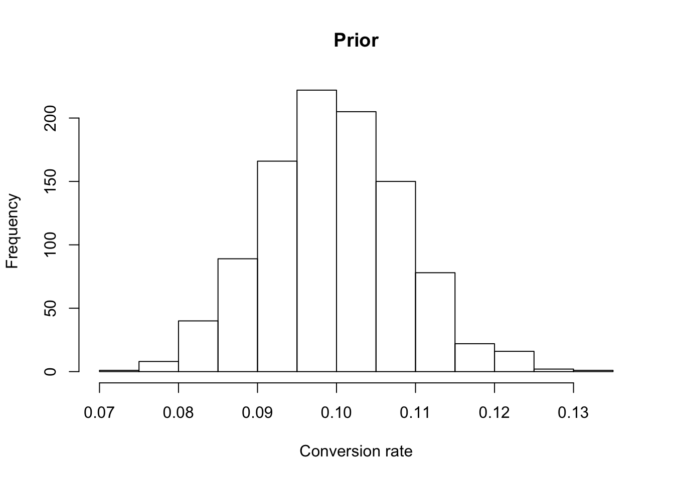
# Stop if chance group a beats group b > 99%
perform_experiment <- function(entrants, a_conv, b_conv,
                               entrants_to_peek_after = 1,
                               prior_a = c(1, 1),
                               prior_b = c(1, 1)) {
  # Step 1: perform experiment for each
  tibble::tibble(
    group_a = rbinom(entrants/2, 1, prob = a_conv),
    group_b = rbinom(entrants/2, 1, prob = b_conv)
  ) %>%
    # https://en.wikipedia.org/wiki/Conjugate_prior#Discrete_distributions
    # see the formula for posterior hyperparameters.
    mutate(group_a_conv_rate_beliefs = map2(cumsum(group_a), 1:n(),
                                            function(x, y) {
                                              rbeta(1e3, x + prior_a[[1]], y - x + prior_b[[2]])
                                            })) %>%
    mutate(group_b_conv_rate_beliefs = map2(cumsum(group_b), 1:n(),
                                            function(x, y) {
                                              rbeta(1e3, x + prior_b[[1]], y - x + prior_b[[2]])
                                            })) %>%
    mutate(belief_a_better = map2_dbl(group_a_conv_rate_beliefs, group_b_conv_rate_beliefs,
                                      function(x, y) {
                                        mean(x > y)
                                      })) %>%
    pull(belief_a_better) -> beliefs_a_better

  beliefs_a_better[
    seq_len(length(beliefs_a_better)) %%
      entrants_to_peek_after == 0] %>%
    max()
}
Let’s assume an experiment of 10k entrants, Group A has a conversion rate of 10%, and Group B has a conversion rate of 10.2%. If we run this experiment 1k times, how often will we see Group A exhibit data that leads us to believe with 99% certainty (under some conditions) it’s the better group?
No prior info
First let’s see what happens if we choose a uniform prior and peek every time,
proc.time <- Sys.time()
# Perform 1k experiments assuming 2% lift of B
parallel::mclapply(seq_len(1e3), function(x) {
  perform_experiment(1e4, 0.1, 0.102, entrants_to_peek_after = 1,
                     prior_a = c(1, 1), prior_b = c(1, 1)) }, mc.cores = 4) %>%
  unlist() -> results
Sys.time() - proc.time
## Time difference of 5.868066 mins# "Type 1 Error" if a dichotomous rule is forced on us
table(results >= 0.99) / length(results)##
## FALSE TRUE
## 0.847 0.153results %>%
as_tibble() %>%
ggplot(aes(x = value)) +
geom_histogram(binwidth = 0.01, colour = "black") +
geom_vline(xintercept = 0.99, colour = "red") +
ggtitle("Histogram of worst case belief a is better\npeeking after every entrant")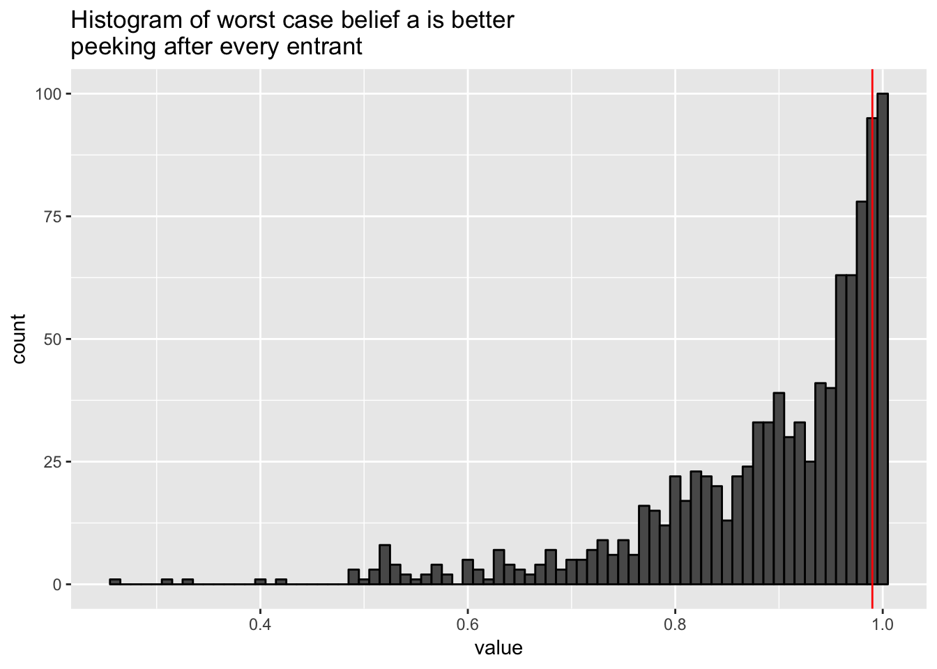
Yikes, 15% of the time we selected Group A (10% vs. Group B’s 10.2%).
Introduce prior
Now I’ll introduce a prior equivalent to seeing 2k entants convert at 10% (a bit of prior info, not an unreasonable amount).
proc.time <- Sys.time()
# Perform 1k experiments assuming 2% lift of B
parallel::mclapply(seq_len(1e3), function(x) {
  perform_experiment(1e4, 0.1, 0.102, entrants_to_peek_after = 1,
                     prior_a = c(1e3*0.1, 1e3*0.9),
                     prior_b = c(1e3*0.1, 1e3*0.9)) }, mc.cores = 4) %>%
  unlist() -> results
Sys.time() - proc.time
## Time difference of 5.854718 mins# "Type 1 Error" if a dichotomous rule is forced on us
table(results >= 0.99) / length(results)##
## FALSE TRUE
## 0.973 0.027results %>%
as_tibble() %>%
ggplot(aes(x = value)) +
geom_histogram(binwidth = 0.01, colour = "black") +
geom_vline(xintercept = 0.99, colour = "red") +
ggtitle("Histogram of worst case belief a is better\npeeking after every entrant")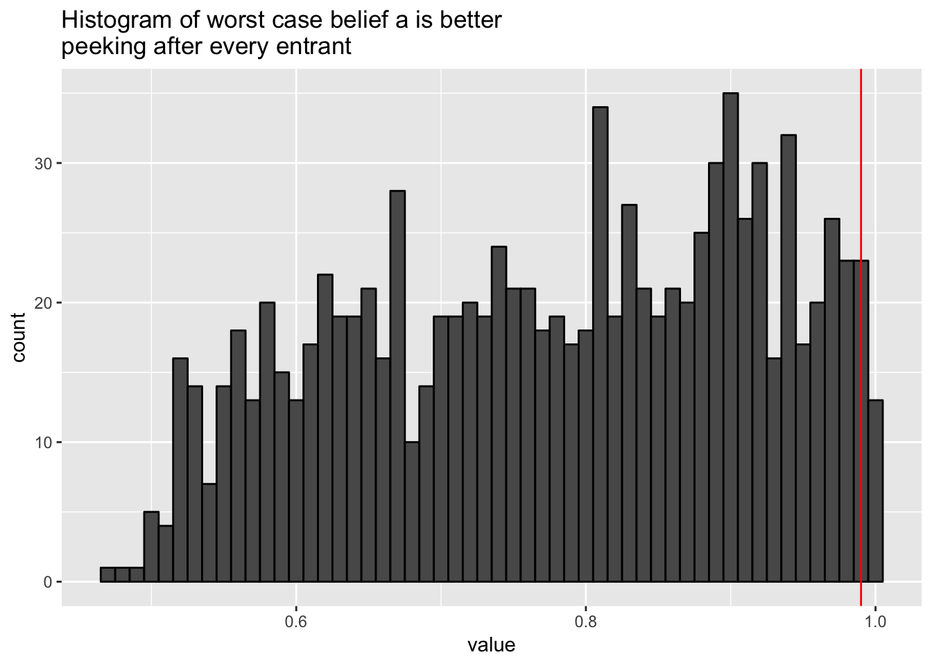
And if we peek after every 100 entrant, or 100 times during each 10k-entrant experiment?
proc.time <- Sys.time()
# Perform 1k experiments assuming 2% lift of B
parallel::mclapply(seq_len(1e3), function(x) {
  perform_experiment(1e4, 0.1, 0.102, entrants_to_peek_after = 100,
                     prior_a = c(1e3*0.1, 1e3*0.9),
                     prior_b = c(1e3*0.1, 1e3*0.9)) }, mc.cores = 4) %>%
  unlist() -> results
Sys.time() - proc.time
## Time difference of 5.892524 mins# "Type 1 Error" if a dichotomous rule is forced on us
table(results >= 0.99) / length(results)##
## FALSE TRUE
## 0.989 0.011results %>%
as_tibble() %>%
ggplot(aes(x = value)) +
geom_histogram(binwidth = 0.01, colour = "black") +
geom_vline(xintercept = 0.99, colour = "red") +
ggtitle("Histogram of worst case belief a is better\npeeking after every 100 entrants (100 times)")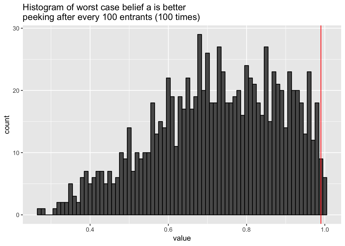
And if we peek just twice during the 10k-entrant experiment?
proc.time <- Sys.time()
# Perform 1k experiments assuming 2% lift of B
parallel::mclapply(seq_len(1e3), function(x) {
  perform_experiment(1e4, 0.1, 0.102, entrants_to_peek_after = 5000,
                     prior_a = c(1e3*0.1, 1e3*0.9),
                     prior_b = c(1e3*0.1, 1e3*0.9)) }, mc.cores = 4) %>%
  unlist() -> results
Sys.time() - proc.time
## Time difference of 5.877045 mins# "Type 1 Error" if a dichotomous rule is forced on us
table(results >= 0.99) / length(results)##
## FALSE
## 1results %>%
as_tibble() %>%
ggplot(aes(x = value)) +
geom_histogram(binwidth = 0.01, colour = "black") +
geom_vline(xintercept = 0.99, colour = "red") +
ggtitle("Histogram of worst case belief a is better\npeeking after every 5,000 entrants (2 times)")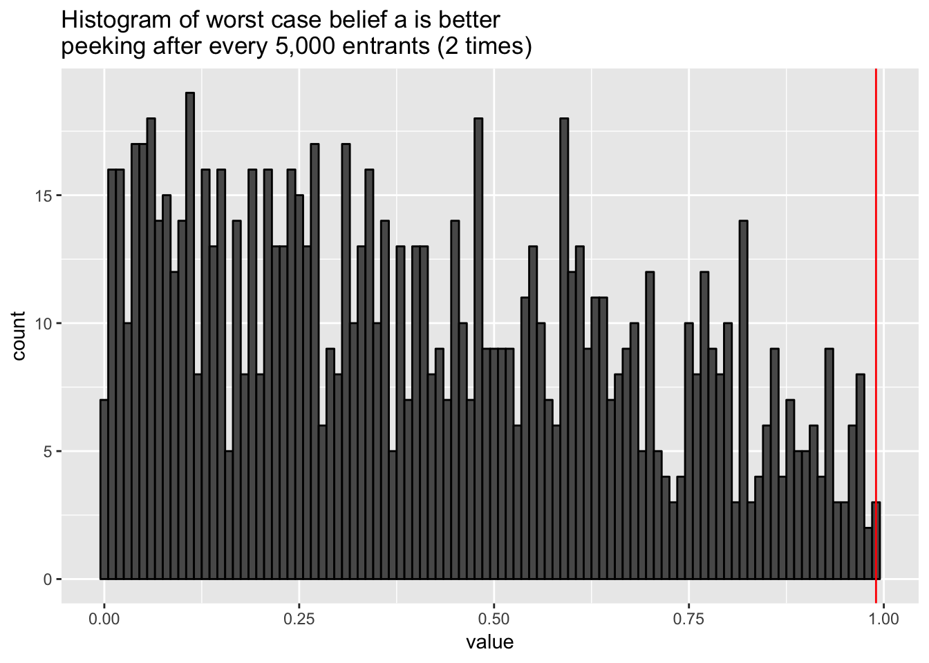
For many tasks, I think these error rates would be acceptable. If needed we can peek and feel confident that if our assumptions are accurate we’re not incurring an unacceptable amount of type 1-like decision risk.