How to speed up experiments using pre-treatment variables
No matter how big data grows, we never seem to have enough. Why is that? I think one reason is that we always have new ideas to try out in experiments and each experiment starts at n=1.
We always want the results of an experiment yesterday. Faster is better. The temptation to peek is irresistable, but makes experiments more fragile.
Consider these two opposing needs, how can we speed up experiments without sacrificing reliability? Pre-treatment variables.
I learned about pairing and blocking in statistician school, but most of the experiments that I run are “analytic study” design rather than “enumerative study” design. Pre-treatment variables translate the blocking/pairing idea to the analytic study design.
In the following simulation, I illustrate the idea. First I generate data in which a pre-treatment variable has no relationship to the treatment effect, intercept + pretreatment_var + treatment_effect. Next I model the results under three conditions: maximal with the pre-treatment variable and treatment effect fully interacted like intercept + pretreatment_var*treatment_effect, additive with each term adjusted for but without interaction (intercept + pretreatment_var + treatment_effect) and finally unadjusted for (intercept + treatment_effect).
In particular I focus on the size of standard error of the treatment effect in each of the three cases. A smaller treatment effect standard error represents more precision per amount of sample size: a faster experiment. I show in the case of no actual treatment interaction, the method fails safe and produces about the same standard error as the “additive” model.
N <- 1e4

generate_data <- function() {
  tibble(
    intercept = 1,
    pretreatment_var = case_when(rbinom(N, 1, p = 0.5) == 1 ~ 0.5, TRUE ~ -0.5),
    treatment_effect = case_when(rbinom(N, 1, p = 0.5) == 1 ~ 1, TRUE ~ 0),
    discrepancy = rnorm(N),
    y = intercept + pretreatment_var + treatment_effect + discrepancy
  )
}
extract_std_error <- . %>%
tidy() %>%
filter(term == "treatment_effect") %>%
pull(std.error)seq_len(1e2) %>%
map_dbl(~ generate_data() %>%
lm(y ~ treatment_effect*pretreatment_var, data = .) %>%
car::deltaMethod("treatment_effect") %>%
tidy() %>%
filter(column == "SE") %>% pull(mean)) %>%
ecdf() %>%
plot(col = "green", lwd = 3, xlim = c(0.019, 0.023),
main = "std.error of treatment_effect")
seq_len(1e2) %>%
map_dbl(~ generate_data() %>%
lm(y ~ treatment_effect + pretreatment_var, data = .) %>%
extract_std_error()) %>%
ecdf() %>%
lines(col = "black", lwd = 3)
seq_len(1e2) %>%
map_dbl(~ generate_data() %>% lm(y ~ treatment_effect, data = .) %>% extract_std_error()) %>%
ecdf() %>%
lines(col = "purple", lwd = 3)
legend("topleft", legend = c("maximal", "additive", "unadjusted for"),
col = c("green", "black", "purple"),
lwd = 5)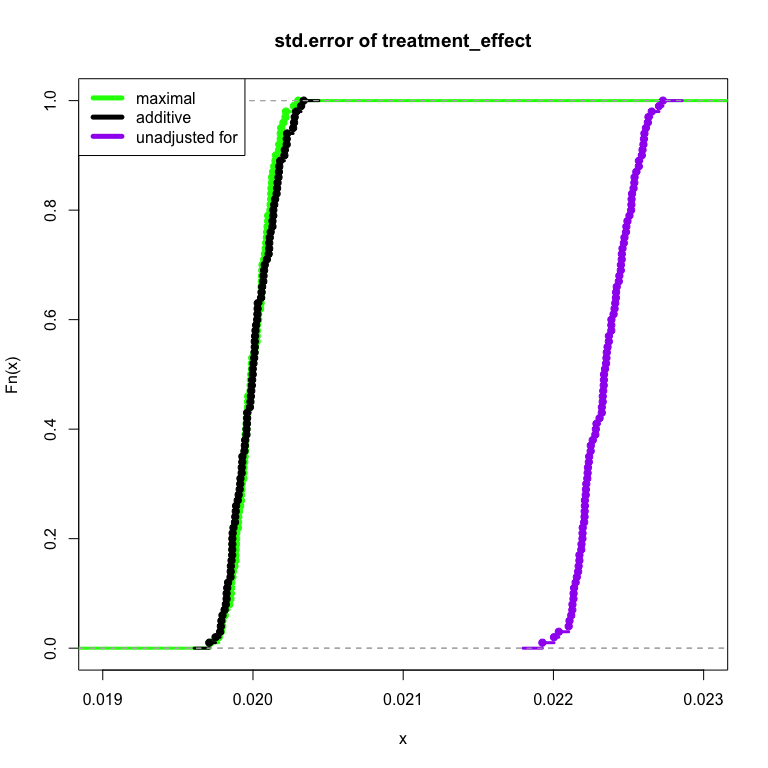
Now let’s assume that not only does the pre-treatment variable affect the outcome, but the treatment also interacts with the pre-treatment variable,
generate_data2 <- function() {
  tibble(
    intercept = 1,
    pretreatment_var = case_when(rbinom(N, 1, p = 0.5) == 1 ~ 0.5, TRUE ~ -0.5),
    treatment_effect = case_when(rbinom(N, 1, p = 0.5) == 1 ~ 1, TRUE ~ 0),
    discrepancy = rnorm(N),
    y = intercept + pretreatment_var*treatment_effect + discrepancy # notice interaction!
  )
}seq_len(1e2) %>%
map_dbl(~ generate_data2() %>%
lm(y ~ treatment_effect*pretreatment_var, data = .) %>%
car::deltaMethod("treatment_effect") %>%
tidy() %>%
filter(column == "SE") %>% pull(mean)) %>%
ecdf() %>%
plot(col = "green", lwd = 3, xlim = c(0.019, 0.023),
main = "std.error of treatment_effect")
seq_len(1e2) %>%
map_dbl(~ generate_data2() %>%
lm(y ~ treatment_effect + pretreatment_var, data = .) %>%
extract_std_error()) %>%
ecdf() %>%
lines(col = "black", lwd = 3)
seq_len(1e2) %>%
map_dbl(~ generate_data2() %>% lm(y ~ treatment_effect, data = .) %>% extract_std_error()) %>%
ecdf() %>%
lines(col = "purple", lwd = 3)
legend("topleft", legend = c("maximal", "additive", "unadjusted for"),
col = c("green", "black", "purple"),
lwd = 5)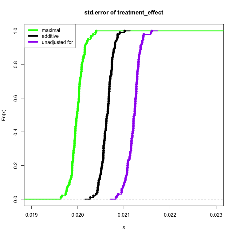
Voila! The pre-treatment maximal fully-interacted model is able to take advantage of the relationship of the pre-treatment variable, our treatment and the outcome. The result is that the model measures information in a more efficient manner. The necessary sample size to achieve the same amount of treatment effect precision is made smaller. The technique can be used to speed up experiments as well as provide deeper understandings of how our treatment performs (through investigation of the interaction).
If you’d like to read more about pre-treatment variables, I’d recommend starting with Chapter 9 of Andrew Gelman and Jennifer Hill’s Data Analysis Using Regression and Multilevel / Hierarchical Models.