Generating zero-inflated negative binomial random numbers
Zero-inflated count data are pretty much everywhere. In fact there are typically many more processes going on in a given count dataset than zero-inflation. Zero-inflation itself may be the realization of serveral processes. These are but one set of random numbers generated from a homogenous zero-inflated negative binomial spec. Whether it’s worth the effort to tease out finer mixtures is a use-case dependent decision. Happy generating!
set.seed(1)
# install.packages('pscl')
suppressPackageStartupMessages({ library(tidyverse); library(reshape2); library(pscl) })
rzinb <- function(n, size, mu, proportion_zero) {
fake_data <- rep(NA_real_, n)
fake_data[which(rbinom(n, 1, prob = proportion_zero) == 0)] <- 0 # set the 0s
nb_fake_data <- rnbinom(n, size = size, mu = mu) # generate a full set of nbs
# fill in spaces left by 0s mask
fake_data[is.na(fake_data)] <- nb_fake_data[is.na(fake_data)]
return(fake_data)
}seq_len(300) %>%
map(function(i) {
N <- 400
X <- rnorm(N)
x <- rzinb(n = N,
size = 1,
mu = exp(1 + X * 0.5),
proportion_zero = 0.5) %>%
tibble(y = .) %>%
mutate(x = X) %>%
pscl::zeroinfl(y ~ x | 1, data = ., dist = "negbin")
output <- x %>% coefficients() %>% as.list()
output$theta <- x$theta
return(output)
}) %>%
map(function(x) { as_tibble(x) }) %>%
bind_rows() %>%
mutate(proportion_zero = plogis(`zero_(Intercept)`)) %>%
select(count_intercept = `count_(Intercept)`, slope = count_x, size = theta, proportion_zero) %>%
reshape2::melt() %>%
ggplot(aes(x = value)) +
geom_density() +
facet_wrap(~ variable, scales = "free")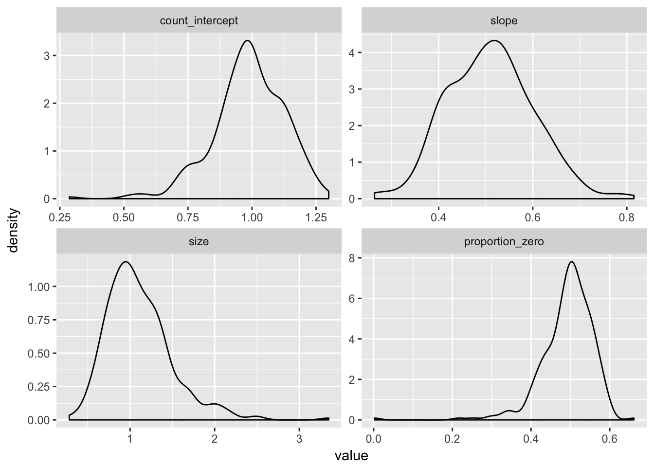
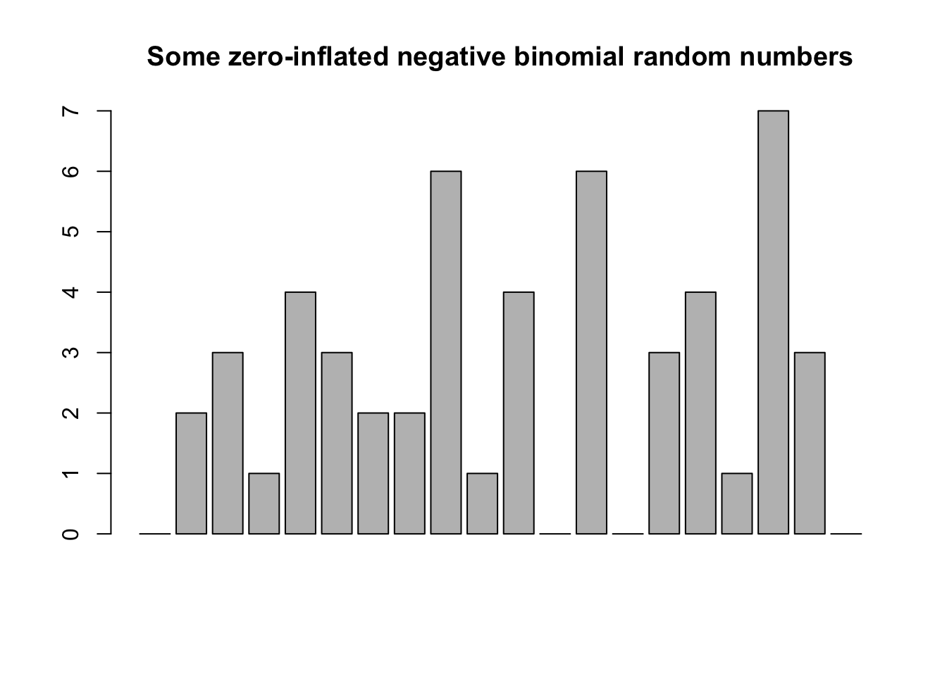
barplot(
  rzinb(20, size = 100, mu = 4, proportion_zero = 0.8),
  main = "Some zero-inflated negative binomial random numbers")