Building on the right-censored Weibull simulation, this article compares Frequentist and Bayesian approaches to estimating Weibull parameters from censored time-to-event data.
Generating Censored Data
library(tidyverse)
library(survival)
library(brms)
library(tidybayes)
library(ggthemes)

rweibull_cens <- function(n, shape, scale) {
  a_random_death_time   <- rweibull(n, shape = shape, scale = scale)
  a_random_censor_time  <- rweibull(n, shape = shape, scale = scale)
  observed_time <- pmin(a_random_censor_time, a_random_death_time)
  censor <- observed_time == a_random_death_time
  tibble(time = observed_time, censor = censor)
}

rweibull_cens(1e4, shape = 1, scale = 10) -> d
Frequentist Approach
d %>%
  survival::survreg(Surv(time, censor) ~ 1, data = .) %>%
  summary()
## Value Std. Error     z      p
## (Intercept)  2.2916     0.0142 161.93  0.000
## Log(scale)  -0.0169     0.0110  -1.54  0.124
##
## Scale = 0.983
## Weibull distribution
## n = 10000
Bayesian Approach with brms
Using brms, a Bayesian model ready to incorporate prior information:
d %>%
  # Note: brms uses opposite 0/1 encoding from survival package
  # 0 for death, 1 for censored
  mutate(censor = if_else(censor == 0, 1, 0)) %>%
  brm(time | cens(censor) ~ 1,
      data = .,
      family = "weibull",
      refresh = 2e3,
      cores = 4) -> bfit

print(bfit, digits = 3)
## Family: weibull
## Formula: time | cens(censor) ~ 1
## Data: . (Number of observations: 10000)
##
## Population-Level Effects:
##           Estimate Est.Error l-95% CI u-95% CI Eff.Sample Rhat
## Intercept    2.285     0.015    2.255    2.316       1994 1.000
##
## Family Specific Parameters:
##       Estimate Est.Error l-95% CI u-95% CI Eff.Sample Rhat
## shape    1.017     0.011    0.995    1.039       2183 1.000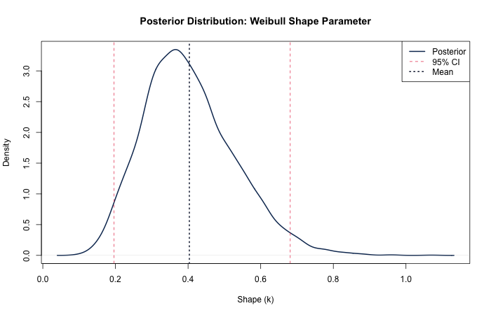
Key Takeaway: Both approaches recover the true parameters well. The Bayesian
approach via brms provides full posterior distributions and naturally incorporates prior
information,
which is especially valuable with small samples or when domain expertise can inform the analysis.