Bernoulli Experiments & Maximum Likelihood with Stan

I'm a big fan of expressing math as code. While it's not as terse, I think it's a lot easier to use to learn statistics. In this post I'll break down a small set (three!) Bernoulli experiments. Binary data is really common in business, so it pays to work through the details.

At the end I'll use Stan to generate a probabilistic estimate of p̂. Markov chain Monte Carlo is overkill for this type of problem, but in order to learn I find it's best to start with simple things.

Generating Bernoulli Experiments

First, I'll generate three Bernoulli experiments with pretend "true" parameter values:

library(rstan)
library(dplyr)

dbernoulli <- function(x, p) dbinom(x, 1, p)
rbernoulli <- function(n, p) rbinom(n, 1, p)
set.seed(1)
N <- 3L
(p <- runif(1))
## [1] 0.2655087

(coin_flips <- rbernoulli(N, p))
## [1] 0 0 1

The Likelihood Function

The most crucial part of doing high quality statistics is to understand how to create and calculate a function that is at worst proportional to the probability of the observed data. This is the likelihood function.

The Bernoulli PDF is: f(x; p) = p^x × (1 - p)^1-x where x can only take the values 0 or 1.

We evaluate the density at each data point and multiply the terms:

bernoulli_likelihood <- function(p_to_try) {
  prod((function() { dbernoulli(coin_flips[1], p_to_try) })(),
       (function() { dbernoulli(coin_flips[2], p_to_try) })(),
       (function() { dbernoulli(coin_flips[3], p_to_try) })())
}

Manual Bisection Search

bernoulli_likelihood(p_to_try = 0.0001)
## [1] 9.998e-05
bernoulli_likelihood(p_to_try = 0.5)
## [1] 0.125
bernoulli_likelihood(p_to_try = 0.25)
## [1] 0.140625
bernoulli_likelihood(p_to_try = 0.375)
## [1] 0.1464844
bernoulli_likelihood(p_to_try = 0.33)
## [1] 0.1481469
bernoulli_likelihood(p_to_try = 0.3375)
## [1] 0.1481934

We estimated p̂ as ~0.33, not exactly 0.26 but also not bad for only observing three data points! One can always complain that their sample size isn't large enough, but a smarter alternative is to become really good at squeezing the most information out of the least data.

Stan MCMC

Now let's use this as an opportunity to learn some Stan:

model_code <- "
data {
  int N;
  int y[N];
}
parameters {
  real p;
}
model {
  y ~ bernoulli(p);
}"

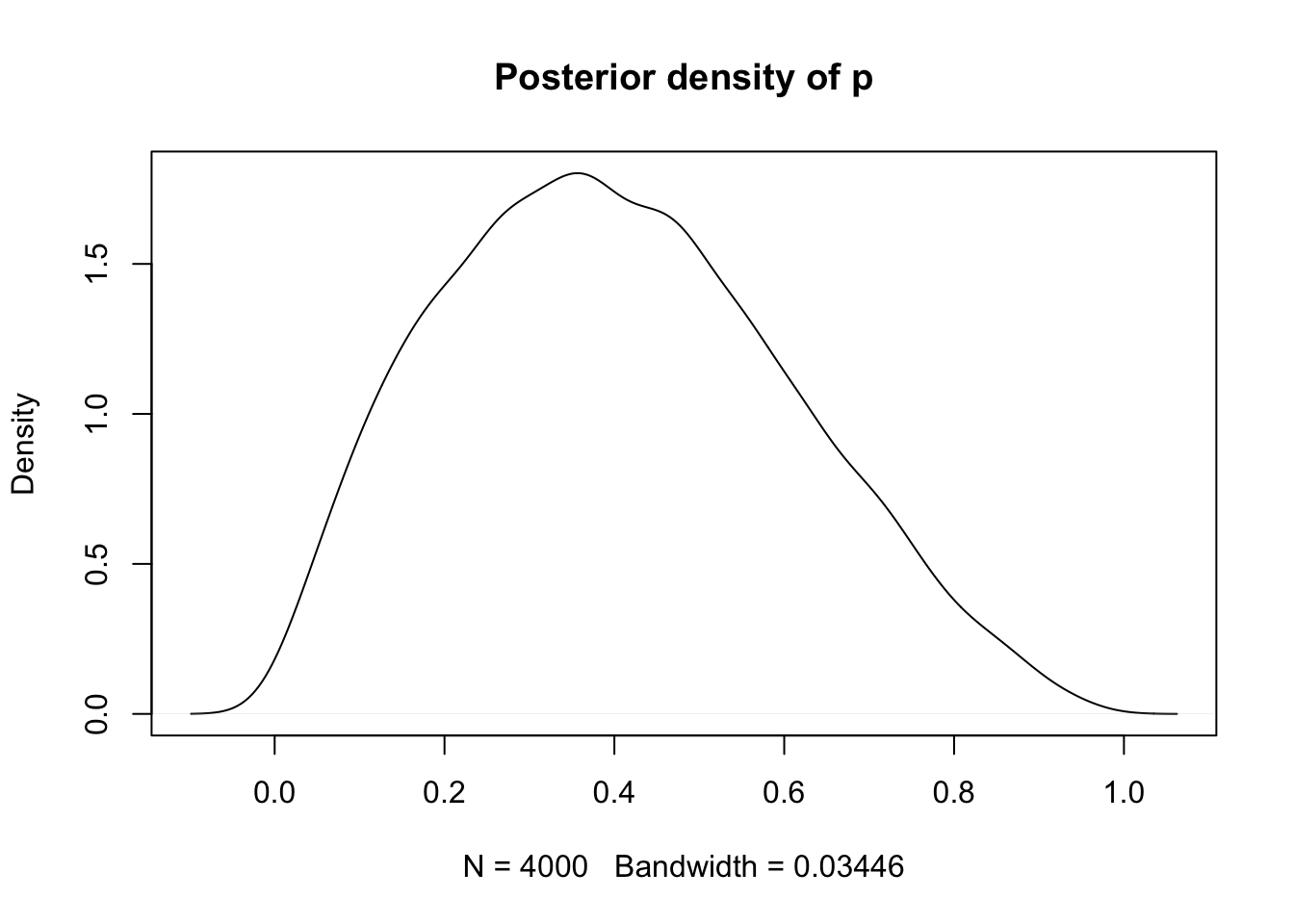
fit <- stan(model_code = model_code,
            data = list(N = N, y = coin_flips))

extract(fit, pars = "p") %>% unlist() %>% density() %>%
  plot(main = "Posterior density of p")