Zero-inflated negative binomial-generalized exponential
I’ve been thinking a lot about how hierarchical models can be used to model, predict and extract useful information from count data. Count data come in all kinds of exotic forms. Like an eye doctor, a statistician can try out different lenses. Some lenses embed other lenses surprisingly. In fact lenses can morph and take subsets (families of distributions). I love the phrase, ‘divining distributions’.
I certainly can’t take credit for this particular divining distribution, that goes to Sirinapa Aryuyuen, Winai Bodhisuwan and Thidaporn Supapakorn. They should be commended for their work.
library(dplyr)
library(ggplot2)
library(purrr)set.seed(1)
# install.packages('pscl')
suppressPackageStartupMessages({ library(tidyverse); library(reshape2); library(pscl) })Here I take my previous less flexible less general lens, the zero-inflated negative binomial and make it into a more flexible “parent” distribution, the zero-inflated negative binomial-generalized exponential, Previously I had parameterized the rzinb function with the mu parameter. For this problem, I swap to the p parameter (there are multiple choices of parameters for this model, pretty neat). The p parameter in a negative binomial is the probability of getting a heads on any given coin flip if size is the number of heads we’re counting.
rzinb <- function(n, size, p, proportion_zero) {
  fake_data <- rep(NA_real_, n)
  fake_data[which(1 - rbinom(n, 1, prob = proportion_zero) == 0)] <- 0 # set the 0s

  # fill in spaces left by 0s mask by generating a full set of nbs
  fake_data[is.na(fake_data)] <- rnbinom(n, size = size, p = p)[is.na(fake_data)]  # only fill in the mask

  return(fake_data)
}
As laid out in this article we can make a random number generator for the generalized exponential distribution,
rge <- function(n, alpha, beta) {
  (-1 / beta)*log(1 - runif(n)^(1/alpha))
}
rge(1e4, 10, 6) %>% mean()
## [1] 0.4888928rge(1e4, 10, 6) %>%
hist(
main = "histogram of rge(1e4, 10, 6)")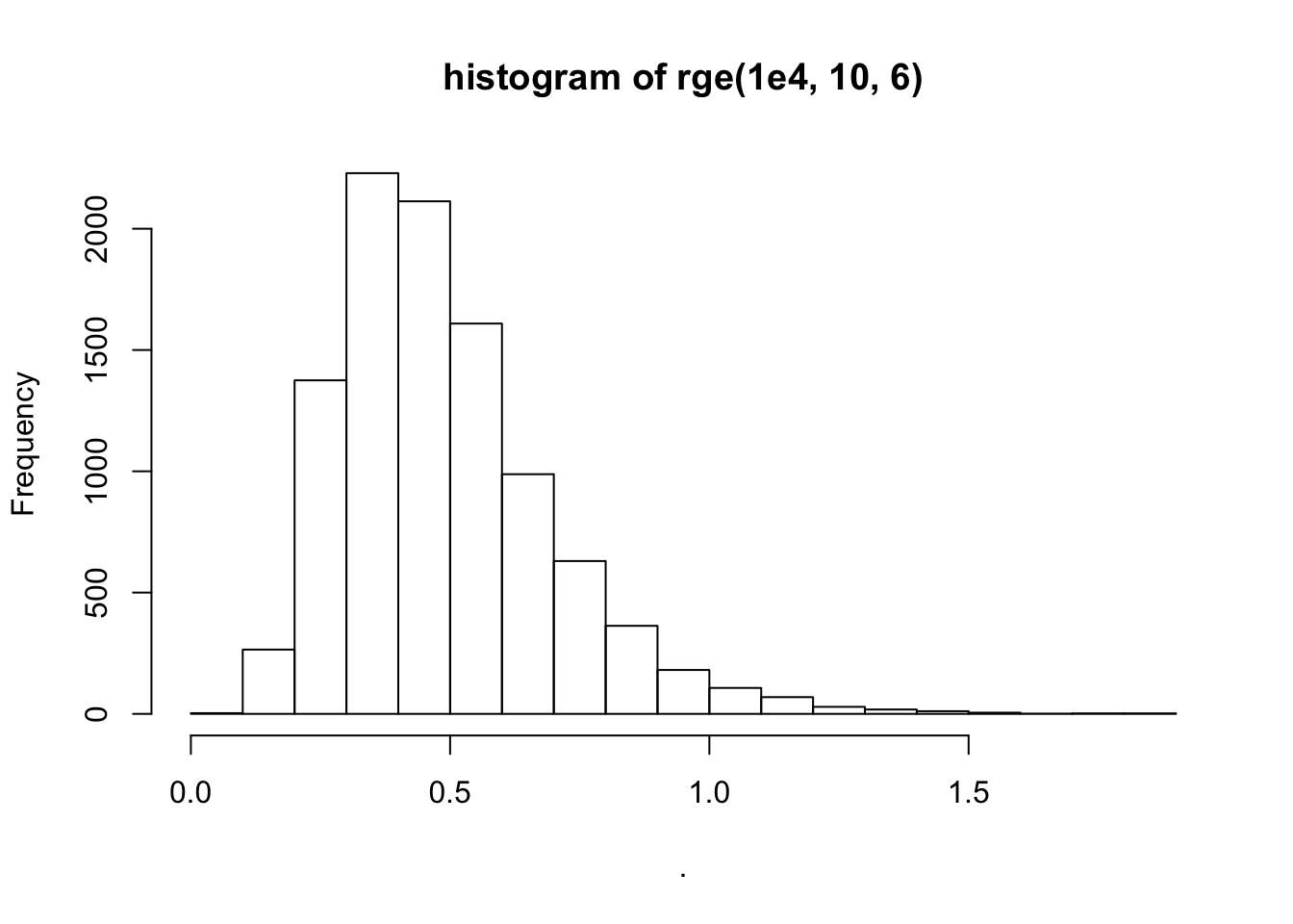
rzinb_generalized_exponential <- function(n, size, alpha, beta, proportion_zero) {
  p <- rge(n, alpha, beta) %>% { exp(-(.)) }
  # message("p is: ", p) # handy for checking that your lambda equals your exp p.
  fake_data <- rep(NA_real_, n)
  fake_data[which(1 - rbinom(n, 1, prob = proportion_zero) == 0)] <- 0 # set the 0s

  # fill in spaces left by 0s mask by generating a full set of nbs
  fake_data[is.na(fake_data)] <- rnbinom(n, size = size, p = p)[is.na(fake_data)]  # only fill in the mask

  return(fake_data)
}
Finally we can see it’s possible to pass a generalized exponential random variable to our usual zero-inflated negative binomial random number generator,
N <- 1e3
rzinb(N, size = 10, p = rge(N, 10, 6) %>% { exp(-.) }, proportion_zero = 0.4) %>%
  ecdf() %>% plot(main = "Zero-inflated nb vs. ZINB-generalized exponential", xlim = c(0, 5))
rzinb_generalized_exponential(N, size = 10, alpha = 10, beta = 6, proportion_zero = 0.4) %>%
  ecdf() %>% plot(add = TRUE, col = "red")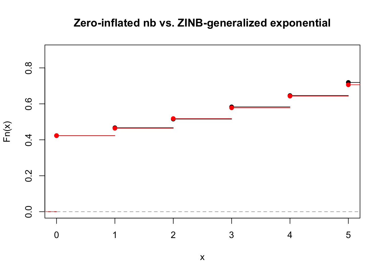
rzinb_generalized_exponential(1000, size = 10, alpha = 10, beta = 6, proportion_zero = 0.4) %>%
  tibble(x = .) %>%
  ggplot(aes(x = x)) +
  geom_histogram(colour = "black", binwidth = 1) +
  coord_cartesian(xlim = c(0, 50)) +
  ggtitle("Zero-inflated negative binomial - generalized exponential") +
  xlab("x") +
  theme_bw()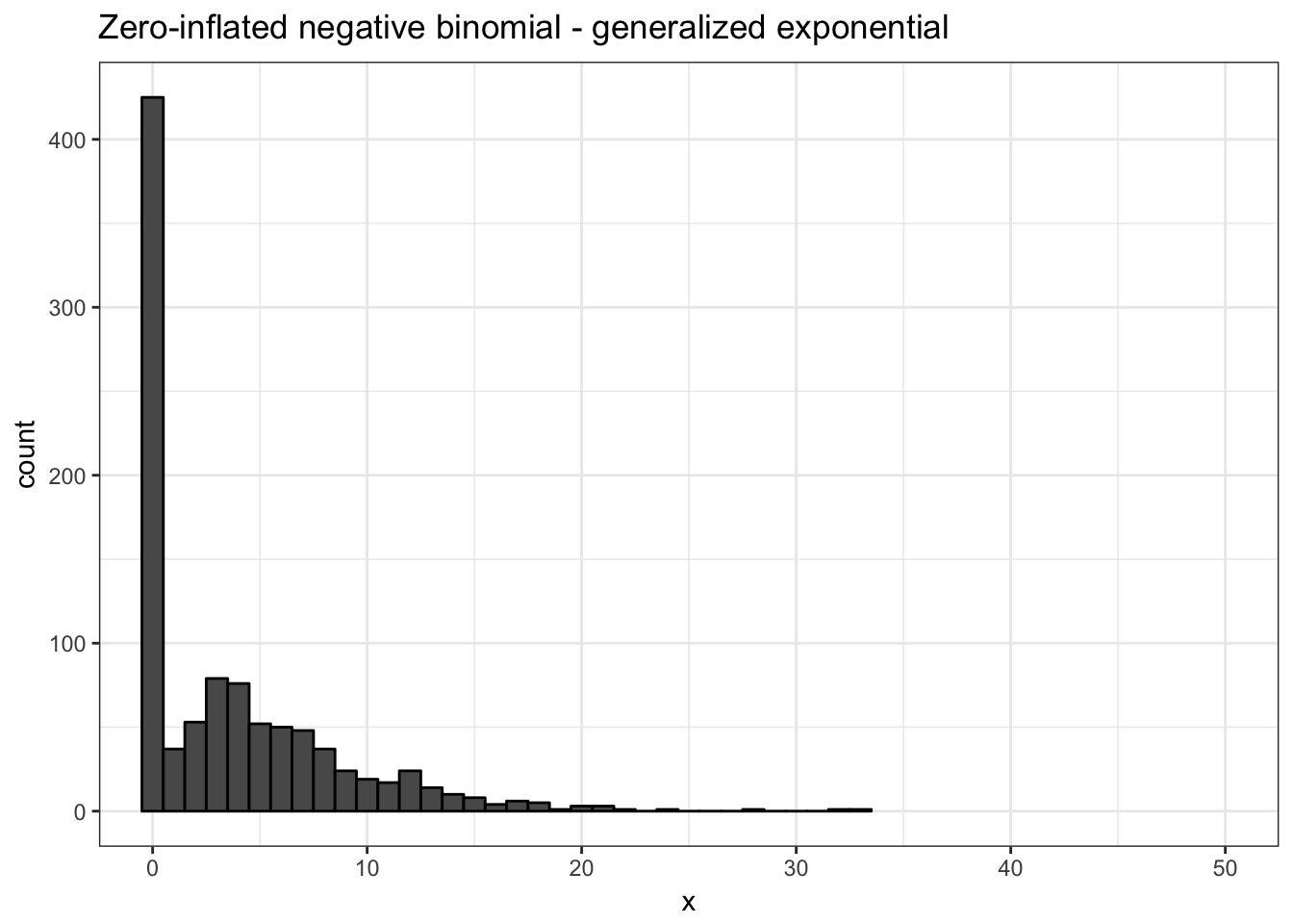
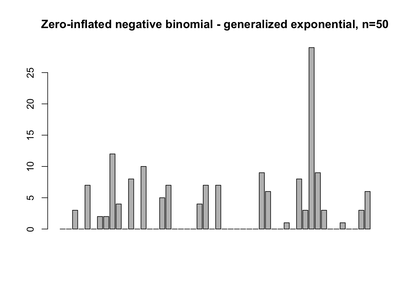
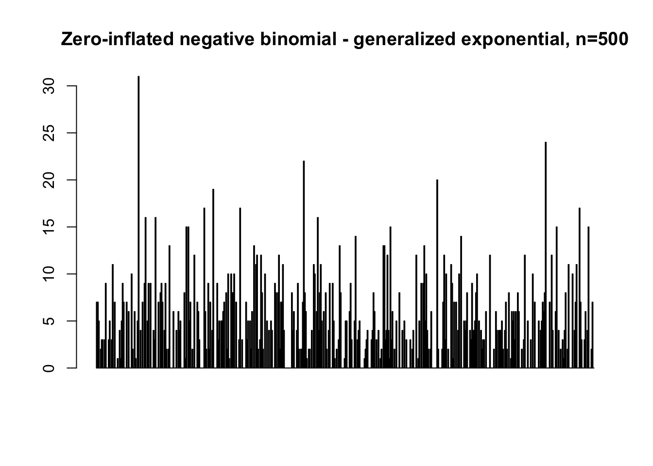
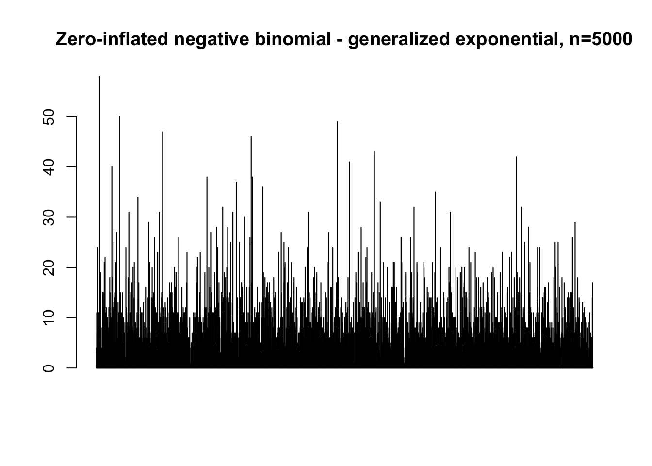
map(c(50, 500, 5000), function(n) {
  rzinb_generalized_exponential(
    n = n, size = 10, alpha = 10, beta = 6, proportion_zero = 0.4) %>%
    barplot(main = paste0("Zero-inflated negative binomial - generalized exponential, n=", n))
})